CS230 • Applied Deep Learning
- Overview
- Comparing to human-level performance
- Error Analysis
- Mismatched Training and Dev Set
- Learning from Multiple Tasks
- Case Study: Building a Speech Recognition System
- Citation
Overview
-
Applied deep learning is not merely about constructing large neural networks and running training loops; it is a systematic discipline concerned with the design, evaluation, and deployment of machine learning systems in real-world environments. While foundational theory equips us with architectures and optimization algorithms, practical success depends on how effectively we:
-
Define goals and metrics — deciding what constitutes success for the model.
In practice this means translating product needs into measurable targets. For example, a medical triage tool might target a recall of at least 0.98 on critical cases, with a maximum average time-to-decision of 50 ms per image. It is often useful to specify multiple operating points (e.g., a “high-sensitivity” and a “balanced” threshold) and to document how thresholds will be chosen post-deployment using calibration curves. When multiple metrics compete (e.g., precision vs. recall), pre-commit to how they will be combined (e.g., \(F_\beta\) with \(\beta>1\) if missing positives is costly), and define guardrail metrics such as fairness slices or latency percentiles.
-
Diagnose performance gaps — identifying whether errors stem from bias, variance, data mismatch, or noise.
Systematic diagnosis decomposes error into: (i) approximation/optimization error visible on the training set (often called “bias”), (ii) generalization gap between train and dev (“variance”), (iii) distribution shift between dev and deployment (“mismatch”), and (iv) residuals due to annotation noise or ill-posed labels. A minimal toolkit includes learning curves (error vs. training size), capacity curves (error vs. model size), ablation tests for regularization, and slice-based evaluation to uncover heterogeneity across subpopulations.
-
Refine training and evaluation pipelines — aligning training, development, and test distributions with deployment needs.
Concretely, design your data pipeline with explicit schemas and versioning for inputs, labels, and augmentations. Keep the development and test sets stationary and representative of the target domain; when the domain drifts, spin a new evaluation set and archive the old one to preserve historical comparability. Automate data quality checks (e.g., label sparsity, class imbalance, feature missingness) and maintain a data card/model card that records collection procedures, known failure modes, and intended use.
-
Leverage human-level performance benchmarks — using them as proxies for Bayes optimal error.
Because the Bayes error is unobservable, carefully selected human baselines provide a practical ceiling. Define which humans matter (novices, experts, committees), how they’re instructed, and how adjudication is performed. Report inter-rater reliability (e.g., Cohen’s \(\kappa\)) so the spread in human labels contextualizes the achievable model performance.
-
Adopt advanced techniques such as transfer learning and multi-task learning to maximize efficiency and adaptability.
Reuse pre-trained representations to shrink data requirements, especially when labels are scarce or expensive. Choose between freezing early layers versus end-to-end fine-tuning based on the size and similarity of your target dataset. In multi-task settings, specify loss weighting (static vs. uncertainty-based) and missing-label handling (masking vs. imputation) to ensure stable joint training.
-
-
In applied settings such as autonomous driving, speech recognition, and medical diagnosis, these considerations often make the difference between a research prototype and a production-ready system. For instance:
- A self-driving car must distinguish between pedestrians, stop signs, and traffic lights under widely varying conditions. Beyond raw accuracy, the system must satisfy strict latency budgets (e.g., \(\le 50\) ms frame-to-decision), fail safely under sensor outages, and support online calibration when weather or lighting changes.
- A voice-activated assistant must function reliably despite accents, background noise, or microphone quality differences. Robustness often comes from targeted augmentation (reverberation, room impulse responses), domain-adaptive fine-tuning, and confidence-based fallback policies to avoid false activations.
- A medical imaging system must generalize across hospitals, imaging devices, and patient populations. Here, data governance, de-identification, harmonization across scanners, and slice-wise calibration are as vital as architecture choice; post-deployment monitoring with drift detectors helps maintain performance as case mix evolves.
-
A recurring theme throughout this chapter is orthogonalization: designing processes so that solving one problem (e.g., bias reduction) does not interfere with another (e.g., variance reduction). By structuring model development into well-defined, independent steps, we can methodically isolate challenges and optimize them with minimal unintended side effects.
-
The sections that follow explore:
- Orthogonalization
- Goal setting and evaluation metrics
- Human-level performance as a benchmark
- Structured error analysis
- Handling mismatched training and deployment data
- Learning across tasks via transfer and multi-task learning
-
Together, these provide a practical toolkit for building robust, scalable, and high-performing deep learning systems.
Orthogonalization
-
In applied machine learning, the principle of orthogonalization refers to designing hyperparameters such that adjusting one does not inadvertently affect others. The term is borrowed from linear algebra, where orthogonal vectors are independent. Similarly, in machine learning, we want independence between hyperparameter effects.
-
Consider a self-driving car: changes in acceleration should not unintentionally alter steering control. Likewise, in machine learning development, we typically pursue four sequential goals:
- Fit the training set well.
- Fit the development (dev) set well.
- Fit the test set well.
- Ensure robustness in the real-world environment.
-
If progress stalls at any stage, the ideal solution is to adjust a dedicated set of knobs for just that stage:
- Training fit: increase capacity (depth/width), improve optimization (learning-rate schedules, better initializations), or enrich data via augmentation; avoid touching regularization strength used to control variance.
- Dev generalization: regularize (weight decay, dropout, mixup), increase data or data diversity, tune early stopping; avoid altering data curation for the evaluation split.
- Test alignment: verify the dev/test sampling and annotation protocols are matched; if they diverge, rebuild the evaluation suite rather than tweaking the model.
- Real-world robustness: add domain adaptation, uncertainty estimation, rejection options, or post-deployment calibration, while holding the core training recipe fixed.
-
This framework allows us to systematically debug model performance. If we fail at step (1), we typically diagnose bias (underfitting). If we succeed at (1) but fail at (2), the issue lies with variance (overfitting). If (2) succeeds but (3) fails, the culprit is data mismatch. Finally, if (3) succeeds but (4) fails, the issue stems from robustness or concept drift in real-world deployment. Clear separation of concerns keeps interventions targeted and reduces unintended regressions elsewhere.
Single number evaluation metric
-
A common problem in practice is choosing between competing models when multiple evaluation metrics are available. For example, in binary classification tasks such as cat vs. non-cat detection, we typically measure both precision and recall:
- Precision (P): the proportion of predicted positive instances that are truly positive. In our cat classifier example, this corresponds to the percentage of images classified as cats that are in fact cats.
- Recall (R): the proportion of actual positive instances that are correctly identified. In this case, the percentage of all cat images that the model correctly labels as cats.
-
The following table shows a comparison of two classifiers (A and B) with respect to precision and recall. Classifier A demonstrates higher recall, while Classifier B achieves higher precision, making the overall choice between them ambiguous without a combined metric.
| Classifier | Precision | Recall |
|---|---|---|
| A | 95% | 90% |
| B | 98% | 85% |
-
Classifier A achieves higher recall, while Classifier B achieves higher precision. Choosing between them is non-trivial because improving precision often comes at the cost of recall, and vice versa.
-
To resolve this, we combine the two metrics into a single-number evaluation metric using the F1 Score, defined as the harmonic mean of precision and recall:
-
The harmonic mean strongly penalizes imbalance; for example, \(P=0.99, R=0.10\) yields \(F1\approx 0.18\), properly flagging an unusable detector when misses are costly. In regulated domains, you may instead use \(F_\beta\) with \(\beta>1\) to weight recall more heavily, or cost-weighted utility when false positives/negatives have asymmetric costs.
-
The following table presents the calculated F1 scores for classifiers A and B, combining their precision and recall into a single performance measure. The results show that Classifier A slightly outperforms Classifier B when evaluated with this balanced metric.
| Classifier | Precision | Recall | F1 Score |
|---|---|---|---|
| A | 95% | 90% | 92.4% |
| B | 98% | 85% | 91.0% |
- Based on the F1 Score, Classifier A is the better option overall. In deployment, however, you would still select a decision threshold that optimizes downstream utility and verify calibration (e.g., using reliability diagrams or expected calibration error) so that predicted probabilities are trustworthy for policy decisions.
Choosing metrics in practice
-
When designing systems, we recommend:
- Define an evaluation metric early. This allows you to establish a clear optimization goal and align data collection with how performance will be judged.
- Separate metric definition from optimization. First decide how performance will be measured, then design optimization strategies. Resist changing the metric mid-experiment unless you also reset comparisons.
- Revisit metrics when needed. If discrepancies arise between development, test, and real-world data, it may be necessary to adjust the metric to better reflect practical requirements, but document all changes and maintain lineage to preserve comparability over time.
-
This separation of concerns prevents over-optimizing toward misleading metrics and ensures long-term model reliability.
Train/dev/test distributions
-
Another critical design choice involves how we partition data into training, development (dev), and test sets. The fundamental principle is that both the dev set and test set should reflect the distribution of data that the system is expected to encounter in deployment.
-
Training set: used to learn parameters.
-
Development set: used for model selection and hyperparameter tuning.
-
Test set: used strictly for final evaluation.
-
The dev and test sets must be sampled from the same distribution, otherwise the dev set ceases to be a reliable proxy for generalization. The test set should be sufficiently large to provide high statistical confidence in performance estimates, particularly when small error differences matter. Estimating confidence intervals (e.g., Wilson intervals for proportions) is good practice when comparing close variants; if intervals overlap strongly, invest in larger evaluation sets or A/B tests.
-
For example, in medical imaging applications, the test set may need to be extremely large because performance differences of even \(0.1\%\) may be significant in real-world terms. In contrast, for tasks such as ad recommendation, smaller test sets may suffice, as large performance gaps are common and easy to detect.
Comparing to human-level performance
-
In applied deep learning, one of the most informative benchmarks is human-level performance. Many tasks—such as image recognition, medical diagnosis, or speech transcription—can be performed by humans with high accuracy. Comparing machine learning systems against human-level benchmarks provides both a reference point and a practical upper bound for performance.
-
In theory, the true limit on achievable accuracy is given by the Bayes optimal error, the lowest possible error rate attainable by any classifier given the underlying data distribution. Because the Bayes optimal error is unobservable, we use carefully measured human-level error as a proxy ceiling. Choose the human baseline deliberately: novice vs. expert, single rater vs. adjudicated panel, and specify the protocol, instructions, and time limits so that the baseline is reproducible and relevant to deployment.
Performance progression over time
-
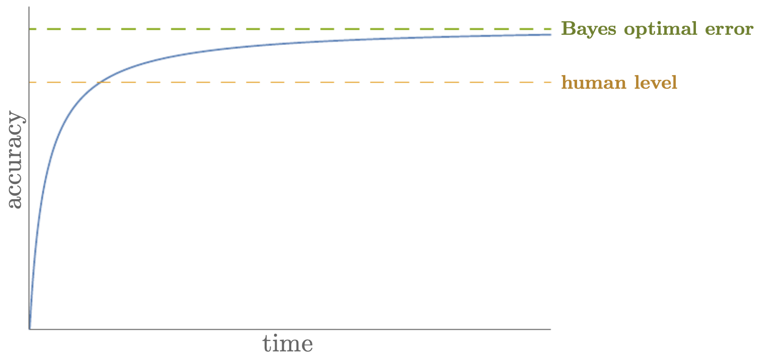
As deep learning models mature on a task, their performance often follows a characteristic trajectory:
- Early stages show rapid improvement as the model learns high-variance but useful features.
- Performance approaches human-level accuracy as representation learning and data scale improve.
- A plateau emerges when remaining error consists largely of irreducible noise, annotation ambiguity, or edge cases that challenge even experts.
-
The following figure visualizes this arc. The curve starts with steep gains, bends as it nears human-level accuracy, and flattens near the Bayes limit, highlighting diminishing returns and the need for better data, labels, or problem reformulation once the curve saturates. Integrating this picture with your roadmap helps decide when to invest in architectural changes versus dataset and labeling improvements.
Quantifying avoidable bias and variance around a human baseline
-
Let \(E_{\text{human}}\) be the measured human error on a representative evaluation set, \(E_{\text{train}}\) the model’s training error, and \(E_{\text{dev}}\) the development error. Two gaps are particularly diagnostic:
- Avoidable bias: \(E_{\text{train}} - E_{\text{human}}\). Large values suggest underfitting or optimization issues; interventions include more capacity, better pretraining, longer schedules, or richer features.
- Variance: \(E_{\text{dev}} - E_{\text{train}}\). Large values indicate overfitting; interventions include regularization (weight decay, dropout, mixup), stronger data augmentation, or more diverse data.
-
When the model surpasses human-level performance (\(E_{\text{dev}} < E_{\text{human}}\)), the bottlenecks often shift from core accuracy to robustness, calibration, fairness across subgroups, and interpretability.
Designing a trustworthy human baseline
- Define the human cohort: novices, typical practitioners, or experts. If deployment replaces or assists experts, benchmark against adjudicated expert consensus, not a single rater.
- Measure reliability: report inter-rater agreement (e.g., Cohen’s \(\kappa\), Fleiss’ \(\kappa\)) and confidence intervals. High disagreement implies that a portion of error is label noise rather than model failure.
- Standardize conditions: give raters the same inputs and time limits the model will see; document instructions and tie-breaking rules. If the model uses multimodal inputs, ensure humans see a comparable information set.
- Adjudication protocol: when multiple raters disagree, use arbitration or majority vote to estimate a practical ceiling and to construct cleaner evaluation labels.
Choosing objectives near and beyond human-level performance
-
When below human level: prioritize reducing avoidable bias and variance. Useful tools include curriculum learning, self-supervised or contrastive pretraining, and targeted data collection in high-error slices. Explicitly track the gaps
\[\Delta_{\text{bias}} = E_{\text{train}} - E_{\text{human}}, \qquad \Delta_{\text{var}} = E_{\text{dev}} - E_{\text{train}},\]and reallocate effort toward the larger term.
-
When at human level: gains usually come from better labels (consensus labeling, label smoothing with soft targets), richer context (longer temporal windows, higher resolution), or problem decompositions that reduce ambiguity (e.g., two-stage systems with an assistive triage).
-
When beyond human level: emphasize calibration and decision quality. Evaluate expected utility under application-specific costs, check probability calibration (e.g., expected calibration error), and implement abstention or referral policies when uncertainty is high. At this stage, invest in fairness diagnostics across cohorts; small average gains can mask subgroup regressions.
Worked examples and practical implications
-
Suppose a dermatology classifier yields \(E_{\text{train}}=6\%\), \(E_{\text{dev}}=9\%\), while a panel of board-certified dermatologists has \(E_{\text{human}}=4\%\). Here, \(\Delta_{\text{bias}}=2\%\), \(\Delta_{\text{var}}=3\%\). Start with bias reduction (capacity, pretraining on large image corpora, longer schedules) until \(E_{\text{train}}\) approaches \(4\%\), then switch to variance reduction (augmentations such as stain normalization, mixup, stronger weight decay). If a new adjudicated panel yields \(E_{\text{human}}=3.2\%\), update the target ceiling and reassess.
-
Conversely, in ad click-through prediction, a model might achieve \(E_{\text{dev}}=12.0\%\) log loss while human heuristics effectively saturate at far worse performance. Being “beyond human” does not eliminate the need for careful calibration and A/B testing; optimize for downstream metrics (lift, ROI) and validate across traffic segments to avoid regressions hidden by aggregate improvements.
Takeaways
- Human-level error is a practical stand-in for the Bayes limit; define it carefully and measure it rigorously.
- Decompose gaps relative to this baseline into avoidable bias and variance to target interventions efficiently.
- Near and beyond human-level performance, the focus naturally shifts toward calibration, robustness, subgroup equity, and decision-theoretic optimization rather than raw accuracy alone.
Error Analysis
-
Error analysis is a systematic process for diagnosing failure modes in machine learning systems. Rather than relying on intuition or anecdotal testing, error analysis provides a quantitative framework to identify which improvements will yield the greatest reduction in overall error. This is especially crucial when resources (time, data collection, labeling) are limited, as it ensures that effort is directed where it has the most impact.
-
Suppose we have a cat classifier with a 10% error rate while the estimated Bayes optimal error is 2%. The immediate question becomes: what types of errors make up the remaining 8% gap, and which categories are worth addressing first?
Identifying Key Error Sources
-
Begin by hypothesizing which categories of inputs might be confusing the classifier. For example:
- Dogs mislabeled as cats.
- Images of large cats (lions, panthers) mistaken for domestic cats.
- Low-quality or blurry images.
-
To evaluate these hypotheses, inspect a representative sample of misclassified images. For each image, record which error categories apply. The resulting counts can be summarized in a table.
-
For instance, if there are 100 misclassified images and 50 involve dogs, then even perfect dog disambiguation could reduce error from 10% \(\rightarrow\) 5%. Conversely, if only 5 involve dogs, then maximum improvement is 10% \(\rightarrow\) 9.5%, making that effort relatively low yield.
Analyzing Multiple Error Categories
-
Often, multiple categories contribute to the same error. An image could be both blurry and contain a large cat. To capture this, we extend our diagnostic table to allow multiple labels per instance:
-
The following table shows how misclassified images can be categorized into overlapping error sources (dogs, large cats, blur), making clear which categories dominate and which overlap frequently.
| Image | Dog | Great cats | Blurry | Comments |
|---|---|---|---|---|
| 1 | Pitbull ✓ | |||
| 2 | ✓ | ✓ | ✓ | Multiple confounders |
| 3 | ✓ | Rainy day at zoo | ||
| … | … | … | … | … |
| Total % | 8% | 43% | 61% |
- This structured approach helps prioritize interventions. If 61% of errors involve blurry images, then augmenting training data with synthetic blur or collecting more naturally blurry samples may yield the highest payoff.
Cleaning Up Incorrect Labels
-
Another significant error source is labeling noise. Especially in crowd-sourced datasets, mislabeled images can confuse the classifier and distort performance metrics.
-
To account for this, we extend the diagnostic table to include a column for incorrectly labeled data. This highlights whether errors are due to the model itself or the dataset quality.
-
The following table adds an “Incorrectly labeled” column, revealing cases where dataset quality contributes directly to observed error rates.
| Image | Dog | Great cats | Blurry | Incorrectly labeled | Comments |
|---|---|---|---|---|---|
| 98 | ✓ | Cat in background labeled as dog | |||
| 99 | ✓ | ||||
| 100 | ✓ | ✓ | Drawing of a cat mislabeled | ||
| Total % | 8% | 43% | 61% | 6% |
-
Whether to invest in label cleanup depends on scale:
- If mislabeled data contributes only ~0.6% to overall error (6% of 10%), it may not be worth immediate attention.
- But if improvements elsewhere reduce error close to 2–3%, then correcting mislabeled samples becomes critical to push further.
Best Practices
- Quantify error categories rather than relying on intuition.
- Prioritize by potential error reduction ceiling (maximum possible improvement).
- Iteratively refine analysis as interventions shift the error landscape.
- Address mislabeled data selectively, focusing only when it becomes a dominant error source.
- Error analysis thus transforms model improvement from a guesswork-driven process into a structured, high-leverage strategy.
Mismatched Training and Dev Set
-
In many real-world applications, the data distribution used for training is not the same as the one encountered at deployment. This problem, known as data mismatch or distribution shift, often causes models to underperform even when they show strong performance on standard dev and test sets.
-
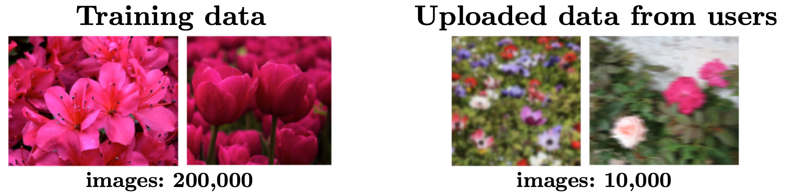
For example, imagine we train an image classifier on 200,000 curated, high-quality training images, but deployment occurs on 10,000 user-uploaded images. The user-uploaded images might differ in background clutter, resolution, or lighting. As a result, even though the model achieves excellent training and dev accuracy on curated data, its performance drops significantly in the real world.
-
The following figure illustrates this contrast between large curated training datasets and smaller, noisier user-uploaded datasets encountered at deployment:
Strategies for Dataset Construction
-
A naïve approach is to mix the curated and user-uploaded data together, shuffle, and split into training/dev/test sets. However, this produces very few user-uploaded examples in the dev/test sets, making them poor indicators of deployment performance.
-
A better approach is:
- Use all curated data (200,000) plus a portion of user-uploaded data (e.g., 5,000) for training.
- Construct the entire dev set and test set from the remaining user-uploaded images (e.g., 2,500 each).
-
This ensures that the dev/test sets accurately reflect deployment data, even if training relies on broader curated datasets. The guiding principle is:
- Train on as much data as possible (even if mismatched).
- Evaluate only on data that matches deployment conditions.
Bias and Variance in the Presence of Mismatch
- Traditional bias-variance decomposition assumes matched distributions, but with mismatch, diagnosis requires an extra tool: the training-dev set.
- Training error: Performance on training data.
- Training-dev error: Performance on a held-out portion of curated data (same distribution as training, never used for training).
- Dev error: Performance on user-uploaded data (deployment distribution).
-
By comparing these three errors:
- If training error ≈ training-dev error « dev error, then mismatch is the main culprit.
- If training error < training-dev error < dev error, then both variance and mismatch contribute.
- If training error is high, bias is also present.
-
This diagnostic framework helps separate model shortcomings from data distribution issues.
Addressing Data Mismatch
- Once mismatch is identified, mitigation strategies include:
-
Targeted data collection
- Gather more deployment-style data.
- Example: if blurry smartphone images dominate errors, intentionally collect blurry training images.
-
Data augmentation
- Artificially simulate deployment conditions by transforming curated data.
- For vision: add blurring, noise, lighting shifts, or occlusions.
- For speech: overlay car noise, café chatter, or microphone distortions.
-
Domain adaptation techniques
- Fine-tune models on a small set of deployment-style samples.
- Apply adversarial methods to align feature distributions across domains.
- Caution: Overusing synthetic augmentation risks overfitting to specific artifacts (e.g., if every audio sample is paired with the same café noise, the model learns the noise, not robustness).
Key Takeaways
- Always ensure dev and test sets reflect deployment distribution.
- Introduce a training-dev set to disentangle variance from mismatch.
- Use data augmentation and targeted collection judiciously to bridge gaps.
- Ultimately, performance on deployment data is the only reliable success metric.
Learning from Multiple Tasks
- Traditional machine learning pipelines often focus on a single, isolated task—for instance, training a network solely to classify cats vs. dogs. However, many real-world applications involve related tasks that share common structure. Leveraging these relationships can make learning more efficient, improve generalization, and reduce data requirements. Two dominant paradigms are transfer learning and multi-task learning.
Transfer Learning
-
Transfer learning is the process of reusing knowledge gained from one task to accelerate or improve learning on a different but related task. In practice, this often means:
- Pretraining a deep neural network on a large, general dataset.
- Adapting it to a specific target task with limited labeled data.
-
Example:
- A CNN trained on ImageNet (1.2M labeled images, 1,000 categories) learns low-level features such as edges, corners, and textures.
- These features are also relevant to medical imaging tasks (e.g., tumor detection in MRI scans).
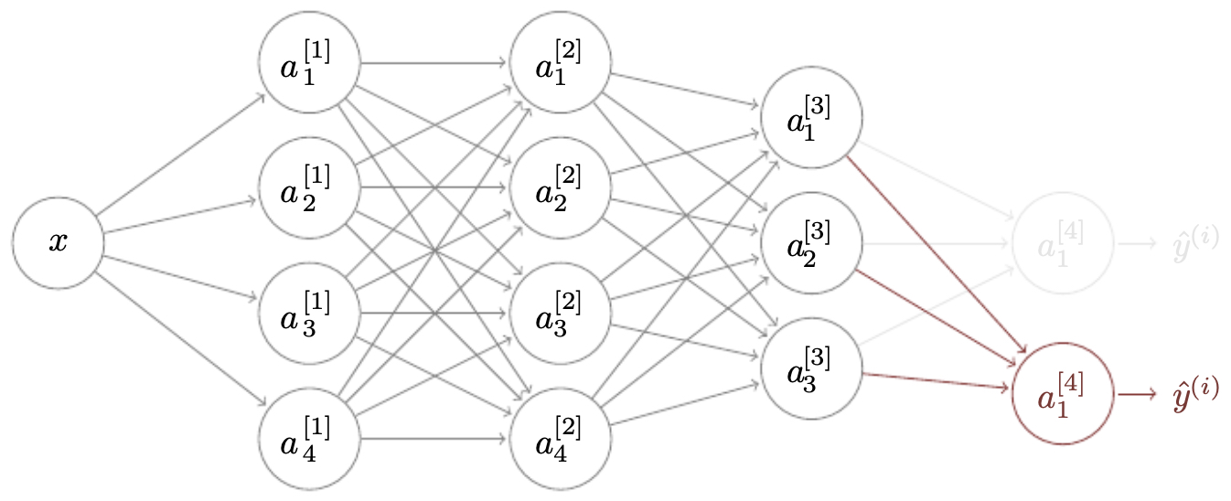
- By reusing pretrained layers and retraining only the task-specific output layers, we achieve strong performance with fewer medical images.
-
The following figure illustrates this workflow: the pretrained model’s feature extraction layers are retained, while the final layers are replaced and reinitialized for the new domain.
-
Key principles of transfer learning:
-
Freezing vs. fine-tuning
- With limited target data, freeze earlier layers and only train the new output layers.
- With abundant target data, fine-tune the entire network for maximal adaptation.
-
Task similarity
- Transfer works best when the source and target tasks share underlying representations (e.g., natural vs. medical images).
-
Initialization of new layers
- Newly added layers should be randomly initialized to prevent bias from the pretrained task.
-
-
Transfer learning is now central across domains:
Multi-Task Learning
-
Multi-task learning (MTL) trains a single neural network to perform several related tasks simultaneously. Instead of separate models, one network shares low-level representations across tasks while having separate heads for each output.
-
Example: A self-driving car system must detect:
- Pedestrians
- Cars
- Stop signs
- Traffic lights
-
Instead of four independent networks, MTL uses a shared backbone plus task-specific outputs. This setup encourages the network to learn general-purpose features that benefit all tasks.
-
Formally, we represent the multi-task label for input \(x^{(i)}\) as a multi-hot vector:
-
If an image contains both a pedestrian and a car, multiple entries can be 1. This differs from softmax classification, where only one class can be active.
-
Advantages of multi-task learning:
- Shared low-level features: Convolutional filters detecting edges, shapes, or textures benefit multiple tasks.
- Regularization via related tasks: Sharing parameters across tasks prevents overfitting to a single objective.
- Data efficiency: Partially labeled samples are still useful—missing labels for one task do not invalidate the sample.
-
Requirements for effective MTL:
- Large datasets to avoid underfitting across multiple outputs.
- Related tasks, so that shared features are beneficial.
- Adequate model capacity, to balance shared vs. task-specific representations.
Takeaways
- Transfer learning leverages pretrained representations to accelerate new tasks—especially powerful in low-data regimes.
- Multi-task learning encourages generalizable feature learning across related tasks, improving efficiency and robustness.
- Both paradigms exemplify a broader movement toward general-purpose learning systems that adapt across domains rather than solving one-off problems.
Case Study: Building a Speech Recognition System
-
To consolidate the principles of applied deep learning, let us consider a real-world, open-ended problem: designing a speech recognition system for an embedded smart chip. The chip will be integrated into lamp products so that users can issue voice commands such as “Hey lamp, turn on” or “Hey lamp, turn off.”
-
This case study illustrates how to apply the concepts of orthogonalization, metric design, error analysis, data augmentation, and regularization to move from a research prototype toward a reliable, production-ready system.
Problem Setup
- Goal: Build a trigger-word detection system that activates upon hearing predefined commands.
- Question: What would you do first when building such a system?
Answer:
-
Conduct a literature review
- Explore existing work on trigger-word detection and keyword spotting.
- Skim broadly (e.g., Graves et al., 2013 on RNNs, Hannun et al., 2014 on Deep Speech) before diving into a handful of highly relevant papers.
-
Engage with experts
- Reach out to authors or practitioners to clarify methodological details.
-
Collect and label data
- For trigger word detection, label the audio so that the end of each trigger word corresponds to
1and all other frames are labeled0. This creates a binary sequence aligned with the audio signal.
- For trigger word detection, label the audio so that the end of each trigger word corresponds to
Error Analysis and Labeling Issues
- Scenario: Suppose the model achieves 99.5% accuracy on the dev set, yet inspection reveals that it always predicts
0s (ignoring the trigger word).
Next steps:
-
Address class imbalance
- Positive examples (trigger words) are rare. Extend the labeling window—e.g., label the final 0.5 seconds of the trigger word as
1s rather than just a single frame.
- Positive examples (trigger words) are rare. Extend the labeling window—e.g., label the final 0.5 seconds of the trigger word as
-
Redefine the evaluation metric
- Accuracy is misleading with imbalanced labels. Instead, use precision, recall, or the F1 score to meaningfully capture detection ability.
Dealing with Class Imbalance
- Scenario: A binary classification problem where 99% of labels are positive. A trivial classifier achieves 99% accuracy by always predicting positive.
Solution:
- Balance evaluation sets so that performance reflects deployment goals.
- Use alternative metrics robust to imbalance: recall, specificity, or AUC (area under the ROC curve).
- This follows the orthogonalization principle: carefully choose metrics (what you measure) independently from optimization (how you train).
Generalization and Data Augmentation
- Scenario: The model performs well on training data but poorly on the dev set.
Solution:
-
Data augmentation
- For speech: superimpose recordings with background noise (cafés, buses, cars).
- This simulates deployment conditions and reduces mismatch between training and real-world data.
- The following figure shows this concept, where clean audio is blended with background noise to better match deployment conditions:
- This directly connects back to Section 4.5 on mismatched data distributions.
Training Efficiency and Regularization
- Scenario: Even with augmentation, the model performs poorly on the dev set, and training times are very long.
Solution:
-
Early stopping
- Monitor dev set performance during training.
- Stop training when accuracy plateaus or degrades, preventing wasted compute cycles.
-
Other efficiency methods
- Batch normalization, dropout, and model pruning can further reduce training time and improve generalization.
Lessons Learned
-
This case study demonstrates how abstract principles translate into practical decisions:
- Orthogonalization: Separate metric choice (e.g., F1 vs. accuracy) from optimization methods.
- Error analysis: Structured diagnosis (e.g., class imbalance) reveals bottlenecks.
- Data mismatch: Data augmentation ensures the dev set reflects deployment.
- Regularization and efficiency: Early stopping and related techniques stabilize training and conserve resources.
-
By systematically applying these methods, even open-ended tasks such as speech recognition become tractable and scalable.
Citation
If you found our work useful, please cite it as:
@article{Chadha2020AppliedDeepLearning,
  title   = {Applied Deep Learning},
  author  = {Chadha, Aman},
  journal = {Distilled Notes for Stanford CS230: Deep Learning},
  year    = {2020},
  note    = {\url{https://aman.ai}}
}