Aman's AI Journal • CS230 • Adversarial Attacks and Defenses

Overview
Adversarial Attacks
Defenses to Adversarial Attacks
Why Are Neural Networks Vulnerable to Adversarial Examples?
Further Readings
Citation

Overview

Neural networks are powerful but fragile. Online platforms increasingly rely on neural network–based classifiers to automatically flag and remove harmful content, such as violent or sexually explicit material. Yet, attackers can circumvent these filters by applying subtle, human-imperceptible perturbations to the input. This phenomenon is known as an adversarial attack.
The vulnerability of neural networks to adversarial perturbations was first identified in 2013 by Szegedy et al.. They demonstrated that it is possible to craft fake datapoints across a variety of domains—images (Szegedy et al., 2013), text (Papernot et al., 2017; Ebrahimi et al., 2018), speech (Carlini & Wagner, 2018), and even structured data (McDaniel et al., 2017)—that can reliably fool state-of-the-art classifiers.
Since then, increasingly powerful attack methods have emerged:
- Carlini & Wagner (C\&W) attacks (Carlini & Wagner, 2017) showed how to design optimization-based attacks that evade many defenses.
- Projected Gradient Descent (PGD) (Madry et al., 2018) became the de facto “universal first-order adversary” and is now a benchmark attack in robustness research.
- AutoAttack (Croce & Hein, 2020) combined multiple strong attacks into a reliable evaluation suite that exposes overly optimistic defense claims.
- Beyond classification, adversarial attacks have expanded to large-scale generative models (e.g., GANs and diffusion models) and multimodal systems (Wei et al., 2022).
Adversarial examples reveal a fundamental paradox: the same linearity and gradient-based properties that make neural networks efficient to train also render them vulnerable to adversarial perturbations. Research in this field remains highly active, with directions ranging from robust training algorithms to certifiable defenses and even theoretical frameworks for understanding adversarial robustness.
Recent advances in defenses include:
- Adversarial training with PGD (Madry et al., 2018), still considered the gold standard for robustness, though computationally expensive.
- Randomized smoothing (Cohen et al., 2019), which provides probabilistic certified robustness guarantees under $L_2$-norm perturbations.
- Certified defenses using convex relaxations (Wong & Kolter, 2018) and interval bound propagation (Gowal et al., 2019).
- Robust pretraining and large-scale models (Xie et al., 2020), which suggest that scaling and data diversity can improve robustness.
As neural networks become integrated into critical applications—autonomous driving, healthcare diagnostics, security systems—the robustness of these models will determine whether AI can be trusted in high-stakes environments. Studying adversarial examples is therefore not just a scientific curiosity but a matter of ensuring the safety and reliability of AI systems.
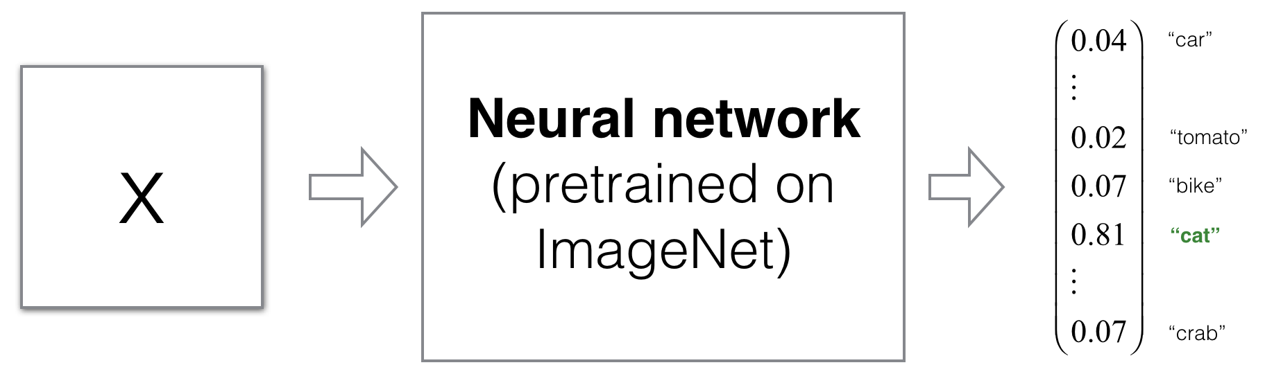
To anchor these ideas, the first visual example makes concrete the notion of a synthetic “fake” datapoint produced entirely by optimization. The pipeline usually starts from either random noise or an unrelated seed and searches, by gradient descent on the input, for an image that a pretrained classifier will assign to a chosen target label with high confidence. The key insight is that no semantic structure recognizable to humans is required; the optimization only needs to navigate decision regions of the model. This underscores how model confidence can be decoupled from human-perceived meaning, motivating robust evaluation beyond raw accuracy.

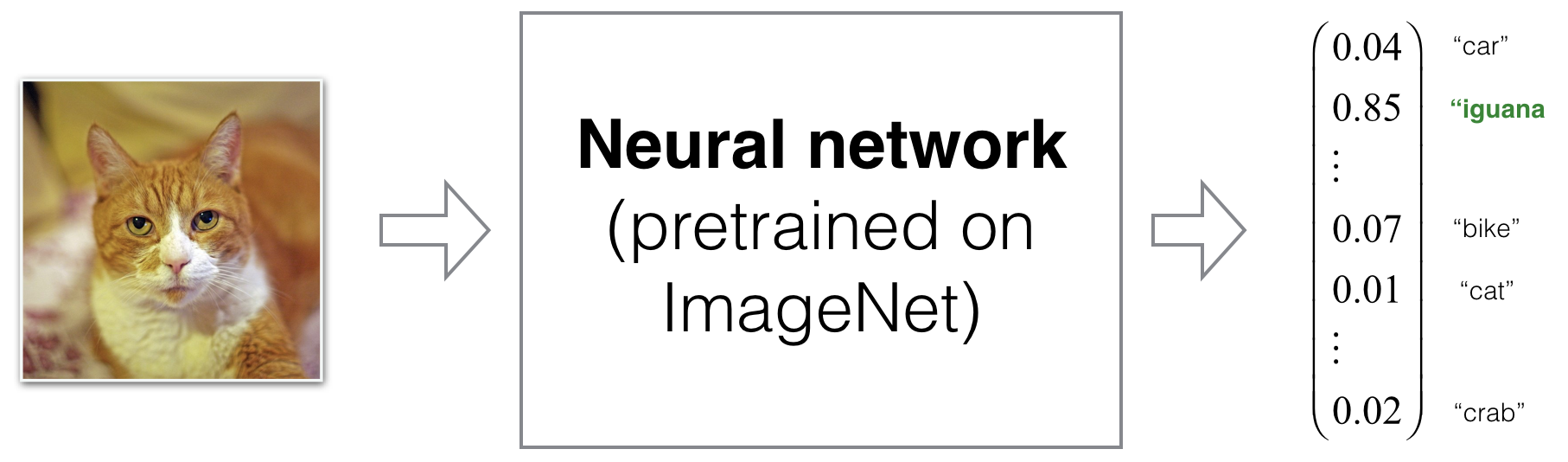
More surprisingly, adversarial perturbations can be designed to be imperceptible. For example, consider an image of a cat. By adding small, carefully calculated pixel-level noise constrained in an $L_p$ norm ball (commonly $L_\infty$ or $L_2$), an attacker can trick a classifier into predicting “iguana” while the perturbed image still looks like a perfectly normal cat to a human observer. Formally, one solves
\[\min_{\delta} \ \mathcal{L}\!\left(f(x+\delta), y_{\text{target}}\right) \quad \text{s.t.} \quad \|\delta\|_p \le \varepsilon,\ \ x+\delta \in [0,1]^d,\]
- where $f$ is the model, $x$ the clean image, $y_{\text{target}}$ the target label, and $\varepsilon$ controls imperceptibility. The constraint ensures the perturbation remains small in the chosen metric, while the loss steers the class decision.
The next figure illustrates this phenomenon end to end: the original cat, an amplified view of the small additive noise (often visualized for pedagogy), and the final adversarial image that appears unchanged to humans yet elicits a confident, incorrect “iguana” prediction. Reading the example alongside the objective above helps connect the visual outcome to the underlying constrained optimization problem.

This has serious real-world implications:
- Autonomous vehicles rely on object detectors to identify pedestrians, vehicles, and traffic signs. An adversarially perturbed “STOP” sign might instead be classified as a “70 mph speed limit” sign, leading to catastrophic accidents.
- Face recognition systems deployed in security settings can be fooled. An unauthorized individual could manipulate their photo so that the system identifies them as an authorized user, granting access.
- Content moderation platforms that screen for prohibited imagery (e.g., violence, explicit content) can be bypassed. Perturbed images evade classifiers, resulting in harmful material slipping past automated filters.
Because of these risks, the study of adversarial examples has become a central research area in modern AI. The field continues to evolve, with ongoing debates about whether true robustness is achievable, or whether adversarial vulnerability is an inherent property of high-dimensional learning systems.

Adversarial Attacks

General Procedure

The process of crafting adversarial examples typically exploits the differentiable structure of neural networks. Consider a convolutional network pre-trained on the ImageNet dataset. The attacker’s objective is to start from a benign input image $x$ and produce a perturbed image $x_{adv}$ such that the model confidently misclassifies it as a chosen target class $y_i$.
At a high level, the adversary reframes the input itself as the optimization variable while holding the network’s parameters fixed. The optimization procedure treats the network as a differentiable mapping from inputs to class scores and backpropagates through the model to compute gradients with respect to the pixels of the input image. This effectively inverts the usual training setup: instead of tuning weights to fit data, the attacker tunes the data to induce a desired misclassification.
The basic procedure can be broken down into the following steps:
1. Forward pass:
  - Select an input $x$ and compute the model’s prediction $\hat{y}$.
2. Define a target loss:
  - Construct a loss function that penalizes deviation from the chosen target class. A simple squared-error loss is:
    \[\mathcal{L}(\hat{y}, y_i) = \frac{1}{2} \, || \hat{y} - y_i ||^2\]
    - where $\hat{y}$ is the prediction vector (e.g., class probabilities) and $y_i$ is the one-hot vector for the target class. In practice, cross-entropy loss is more common, but squared error provides intuition.
3. Iterative optimization on the input:
  - Keep the network weights frozen and update the input image using gradient descent:
    \[x \leftarrow x - \alpha \frac{\partial \mathcal{L}}{\partial x}\]
    - where $\alpha$ is a step size controlling the perturbation strength.
After several iterations, this optimization produces an adversarial example $x_{adv}$ that is highly likely to be classified as the target $y_i$.
This procedure highlights the core vulnerability: neural networks are differentiable end-to-end, which allows attackers to harness the same gradients used for training to craft adversarial perturbations.

State-of-the-Art Attacks

While the above describes the original approach (Szegedy et al., 2013), more advanced attack algorithms have since been developed. These methods refine the optimization objective, incorporate constraints, and improve computational efficiency.
Fast Gradient Sign Method (FGSM) (Goodfellow et al., 2014):
- A single-step method that perturbs the input in the direction of the sign of the gradient:
\[x_{adv} = x + \varepsilon \cdot \text{sign}\left(\nabla_x \mathcal{L}(W, x, y)\right)\]
- FGSM is computationally efficient and widely used both for testing robustness and for generating adversarial examples during adversarial training. The perturbation magnitude is controlled directly by $\varepsilon$, making it interpretable in terms of pixel changes.
Projected Gradient Descent (PGD) (Madry et al., 2018):
- An iterative version of FGSM, PGD applies multiple small updates while projecting the perturbed input back into an $\varepsilon$-ball around the original image:
  \[x_{t+1} = \Pi_{B_\varepsilon(x)} \left( x_t + \alpha \cdot \text{sign}(\nabla_x \mathcal{L}(W, x_t, y)) \right)\]
  - where $\Pi_{B_\varepsilon(x)}$ denotes projection onto the allowed perturbation set. PGD is considered the “universal first-order adversary” and is now the standard benchmark for robustness evaluation.
Carlini & Wagner (C\&W) attack (Carlini & Wagner, 2017):
- A powerful optimization-based attack that reformulates the objective to minimize perturbation magnitude while achieving misclassification. By carefully choosing the loss function and optimization constraints, C\&W can bypass many defenses that stop simpler attacks.
AutoAttack (Croce & Hein, 2020):
- A parameter-free ensemble of strong attacks (including PGD and C\&W variants). AutoAttack has become the standard evaluation suite because it reliably exposes overly optimistic robustness claims.
Beyond classification:
- Modern attacks extend beyond classification to object detection, segmentation, multimodal models (vision-language systems like CLIP), and diffusion models (Wei et al., 2022). These results show that adversarial vulnerability is not an artifact of classifiers alone but is instead a pervasive property of high-dimensional learning systems.

Ensuring Natural-Looking Perturbations

A key challenge is that unconstrained optimization can produce adversarial examples that look like random noise, since the input space is vast. For example, the space of $32 \times 32$ color images is:
\[255^{32 \times 32 \times 3} \approx 10^{7400}\]
- which is astronomically larger than the space of realistic natural images. Without additional constraints, gradient descent may find solutions that succeed mathematically but are obviously unnatural.
To ensure the adversarial example resembles a natural image, the loss can be modified to include a perceptual similarity term:
\[\mathcal{L}(\hat{y}, y_i, x) = \frac{1}{2}||\hat{y} - y_i||^2 + \lambda \, ||x - x_j||^2\]
- where $x_j$ is a chosen reference image (e.g., the original input), and $\lambda$ is a hyperparameter controlling the trade-off between classification success and perceptual similarity. The second term acts as a regularizer that discourages large pixel changes.
The result is an adversarial example that looks like $x_j$ to humans, but the classifier labels it as $y_i$.

In practice, researchers apply additional techniques to keep perturbations imperceptible:
- Gradient clipping: Restricting update magnitudes prevents large pixel changes.
- Norm-based constraints: Perturbations are often bounded by an $L_p$-norm, such as
  \[||x_{adv} - x||_\infty \leq \varepsilon\]
  - ensuring that each pixel is altered by at most $\varepsilon$.
- Early stopping: Once the model confidently predicts the target label, the optimization halts to avoid introducing unnecessary distortion.
These refinements, combined with state-of-the-art attack methods like PGD and AutoAttack, make adversarial examples subtle yet devastatingly effective—posing a persistent challenge for defense research.

Defenses to Adversarial Attacks

The discovery of adversarial examples raised urgent questions about how to safeguard machine learning models in real-world deployments. While numerous defense strategies have been proposed, no single method can guarantee robustness against all possible attacks. Nonetheless, defenses have evolved considerably, from heuristic approaches that rely on simple data augmentations, to sophisticated methods offering certified robustness guarantees.
A useful starting point in discussing defenses is to distinguish between the types of attacks we are trying to defend against.

Types of Attacks

White-box attacks
- The attacker has full knowledge of the model’s architecture, parameters, and gradients.
- This setting is extremely challenging because the adversary can compute exact gradients and tailor perturbations precisely to the model’s weaknesses.
- Example: PGD (Madry et al., 2018) is often evaluated in this setting.
Black-box attacks
- The attacker only has query access: they can submit inputs and observe outputs, but cannot see internals.
- Gradients can be estimated using finite differences:
  \[\frac{\partial \mathcal{L}}{\partial x} \approx \frac{f(x+\varepsilon) - f(x)}{\varepsilon}\]
  - where $f(\cdot)$ is the model’s prediction.
- Due to transferability, adversarial examples crafted for one model often fool another (Papernot et al., 2017), making black-box attacks surprisingly effective in practice.

Early Defense Methods

SafetyNet (adversarial detection)
- Lu et al. (2017) introduced a detector “firewall” network that learns to identify adversarial inputs by monitoring hidden activations.
- Initially promising, but many adaptive attacks later bypassed detection by specifically optimizing to fool both the classifier and the detector.
Adversarial data augmentation
- Generate adversarial examples during training and label them correctly.
- This method helps reshape decision boundaries, making them less sensitive to small perturbations.
- However, generating adversarial data is costly, and robustness often fails when facing unseen attack types.
Adversarial training (FGSM)
- Goodfellow et al. (2014) proposed adding FGSM-generated adversarial examples into training:
  \[\mathcal{L}_{new}(W, x, y) = L(W, x, y) + \lambda L(W, x_{adv}, y)\]
- This approach improved robustness against simple attacks, but it did not hold up against stronger iterative methods like PGD or C\&W.

State-of-the-Art Defenses

Adversarial Training with PGD
- Madry et al. (2018) extended adversarial training using PGD-generated examples.
- PGD training remains the “gold standard” of empirical robustness.
- Its major drawback is computational cost: every training step requires generating adversarial examples with multiple gradient steps, which can be several times slower than standard training.
Randomized Smoothing
- Cohen et al. (2019) showed that adding Gaussian noise during inference transforms a classifier into a smoothed classifier.
- This smoothed model has certified robustness guarantees under $$L_2$-norm perturbations: if the classifier’s prediction remains stable under random noise, it must also be stable under small adversarial perturbations.
- Randomized smoothing scales well to large models and is widely used for certification.
Certified Defenses
- Convex relaxations (Wong & Kolter, 2018) approximate the adversarial optimization problem using convex bounds, providing formal guarantees.
- Interval Bound Propagation (IBP) (Gowal et al., 2019) propagates input intervals through the network to certify robustness in real time.
- These methods offer mathematical guarantees but typically reduce model accuracy and scalability.
Robust Pretraining and Large-Scale Defenses
- Large-scale adversarial pretraining on diverse datasets (Xie et al., 2020) improves robustness compared to training from scratch.
- Recent research combines self-supervised learning with adversarial training, enabling better robustness without prohibitive costs.
Defense Benchmarking
- To counter “broken defenses” (methods that appear robust but collapse under stronger attacks), the community now relies on AutoAttack (Croce & Hein, 2020) to stress-test defenses.
- RobustBench, a public leaderboard, tracks progress and standardizes evaluation protocols.

Computational Considerations

Adversarial training is reliable but can be 10–30× more expensive than standard training for large-scale datasets like ImageNet.
Certified defenses provide guarantees but often sacrifice accuracy and scalability.
Hybrid approaches — such as combining PGD adversarial training with randomized smoothing — are promising directions that aim to balance efficiency with robustness.

Why Are Neural Networks Vulnerable to Adversarial Examples?

The central puzzle of adversarial machine learning is why neural networks are so fragile. Even minuscule perturbations—so small that humans cannot detect them—can completely flip a model’s prediction. Early explanations attributed this fragility to overfitting or the complexity of highly non-linear decision boundaries. However, subsequent work has revealed that the vulnerability of neural networks is more deeply tied to their geometry in high-dimensional spaces and their deliberate design choices (such as linear components and gradient-based optimization).

Example: Adversarial Attack on Logistic Regression

To illustrate the phenomenon in its simplest form, consider a logistic regression model:
\[\hat{y} = \sigma(Wx + b)\]
- where $\sigma(\cdot)$ is the sigmoid function, $x \in \mathbb{R}^{n \times 1}$ is the input, and $W \in \mathbb{R}^{1 \times n}$ is the weight vector. For simplicity, set $b = 0$ and $n = 6$.
Suppose:

\[W = (1, 3, -1, 2, 2, 3), \quad x = (1, -1, 2, 0, 3, -2)^T\]

The model computes:

\[\hat{y} = \sigma(Wx) = \sigma(1 - 3 - 2 + 0 + 6 - 6) = \sigma(-4) \approx 0.27\]

Thus, the model predicts class $y=0$ with 73% confidence.
Now add a perturbation aligned with the sign of the weight vector:

\[x_{adv} = x + \varepsilon \cdot \text{sign}(W)\]

For $\varepsilon = 0.4$:

\[x_{adv} = (1.4, -0.6, 1.6, 0.4, 3.4, -1.6)\]

yielding:

\[\hat{y} = \sigma(Wx_{adv}) = \sigma(0.8) \approx 0.69\]

With this tiny perturbation, the model flips to predict class $y=1$ with 69% confidence.
This simple example demonstrates that adversarial perturbations need not be large. By aligning changes with the weight vector, even small shifts can cumulatively cross the decision boundary.

Key Observations

Why sign perturbations work: Aligning with $\text{sign}(W)$ ensures each feature perturbation contributes positively toward flipping the prediction.
Dimensionality amplifies vulnerability: In high dimensions, the cumulative effect of many small changes is magnified, making models more fragile as input size grows.
Extension to deep networks: For neural networks, the same principle applies, but instead of a weight vector, adversaries exploit gradients of the loss:

\[x_{adv} = x + \varepsilon \cdot \text{sign}\big(\nabla_x \mathcal{L}(W, x, y)\big)\]

This formulation underpins the Fast Gradient Sign Method (FGSM), introduced by Goodfellow et al., 2014.

Why Linearity Makes Networks Fragile

Contrary to early intuition, adversarial vulnerability does not primarily come from non-linear decision boundaries. Goodfellow and colleagues argued that linearity is the culprit:
- Neural networks are designed to be piecewise linear, using activations like ReLU, leaky ReLU, or near-linear regions of sigmoid and tanh.
- Training techniques such as Xavier initialization and Batch Normalization push models toward regimes where gradients propagate cleanly—further encouraging linearity.
- This linearity makes models efficient to optimize, but also easy to exploit: adversaries can use gradient information to steer predictions with surgical precision.
The FGSM attack illustrates this paradox: the same gradient flow that enables backpropagation also enables adversarial manipulation.

Modern Theoretical Perspectives

Curvature of decision boundaries
- Moosavi-Dezfooli et al., 2016 showed that adversarial examples exploit the geometry of decision boundaries, which often lie perilously close to the data manifold in high dimensions.
Universal adversarial perturbations
- Moosavi-Dezfooli et al., 2017 demonstrated that a single carefully designed perturbation vector can fool a model across many different inputs. This global fragility underscores how shallow margins pervade across classes.
Robustness–accuracy trade-off
- Tsipras et al., 2019 argued that accuracy and robustness are inherently at odds: features that maximize classification accuracy may be brittle and non-robust, leaving the model exposed to adversarial attacks.
Non-robust features hypothesis
- Ilyas et al., 2019 suggested that adversarial examples exploit “non-robust features”—statistical patterns that are invisible to humans but predictive in data. Models naturally learn these features, making them fundamentally vulnerable.
Scaling laws and large models
- Larger pretrained models (e.g., Vision Transformers, multimodal systems like CLIP) exhibit improved robustness due to richer representations, but remain vulnerable to adaptive attacks (Wei et al., 2022).
Certified robustness frameworks
- Formal methods (Wong & Kolter, 2018) aim to provide provable guarantees within bounded perturbations, shifting the field from empirical testing to theoretical assurance.

Takeaway

Adversarial examples are not mere artifacts of overfitting or poor training. They are a structural property of high-dimensional learning systems, stemming from:
- Linearity in input–output mappings.
- Heavy reliance on non-robust yet predictive features.
- Decision boundaries that lie uncomfortably close to the data manifold.
- Trade-offs between robustness and accuracy.
This makes adversarial robustness not just a patchable weakness but a fundamental challenge for building reliable AI systems.

Citation

If you found our work useful, please cite it as:

@article{Chadha2020AdversarialAttacks,
  title   = {Adversarial Attacks and Defenses},
  author  = {Chadha, Aman},
  journal = {Distilled Notes for Stanford CS230: Deep Learning},
  year    = {2020},
  note    = {\url{https://aman.ai}}
}

CS230 • Adversarial Attacks and Defenses

Overview

Adversarial Attacks

General Procedure

State-of-the-Art Attacks

Ensuring Natural-Looking Perturbations

Defenses to Adversarial Attacks

Types of Attacks

Early Defense Methods

State-of-the-Art Defenses

Computational Considerations

Why Are Neural Networks Vulnerable to Adversarial Examples?

Example: Adversarial Attack on Logistic Regression

Key Observations

Why Linearity Makes Networks Fragile

Modern Theoretical Perspectives

Takeaway

Further Readings

Foundational Work

Core Attack and Defense Methods

Survey Papers

Domain-Specific Vulnerabilities

Modern Theoretical Perspectives

Emerging Directions

Citation

Overview

Adversarial Attacks

General Procedure

State-of-the-Art Attacks

Ensuring Natural-Looking Perturbations

Practical Refinements

Defenses to Adversarial Attacks

Types of Attacks

Early Defense Methods

State-of-the-Art Defenses

Computational Considerations

Why Are Neural Networks Vulnerable to Adversarial Examples?

Example: Adversarial Attack on Logistic Regression

Key Observations

Why Linearity Makes Networks Fragile

Modern Theoretical Perspectives

Takeaway

Further Readings

Foundational Work

Core Attack and Defense Methods

Survey Papers

Domain-Specific Vulnerabilities

Modern Theoretical Perspectives

Emerging Directions

Citation