CS229 • Reinforcement Learning and Adaptive Control
- Overview
- Markov decision processes
- Value iteration and policy iteration
- Learning a model for an MDP
- Continuous state MDPs
- References
- Citation
Overview
- In this topic, we cover reinforcement learning and adaptive control. In supervised learning, we saw algorithms that tried to make their outputs mimic the labels \(y\) given in the training set. In that setting, the labels gave an unambiguous “right answer” for each of the inputs \(x\). In contrast, for many sequential decision making and control problems, it is very difficult to provide this type of explicit supervision to a learning algorithm. For example, if we have just built a four-legged robot and are trying to program it to walk, then initially we have no idea what the “correct” actions to take are to make it walk, and so do not know how to provide explicit supervision for a learning algorithm to try to mimic.
- In the reinforcement learning framework, we will instead provide our algorithms only a reward function, which indicates to the learning agent when it is doing well, and when it is doing poorly. In the four-legged walking example, the reward function might give the robot positive rewards for moving forwards, and negative rewards for either moving backwards or falling over. It will then be the learning algorithm’s job to figure out how to choose actions over time so as to obtain large rewards.
- Reinforcement learning has been successful in applications as diverse as autonomous helicopter flight, robot legged locomotion, cell-phone network routing, marketing strategy selection, factory control, and efficient web-page indexing. Our study of reinforcement learning will begin with a definition of the Markov decision processes (MDP), which provides the formalism in which RL problems are usually posed.
Markov decision processes
- A Markov decision process is a tuple \(\left(S, A,\left\{p_{s a}\right\}, \gamma, R\right)\), where:
- \(S\) is a set of states. (For example, in autonomous helicopter flight, \(S\) might be the set of all possible positions and orientations of the helicopter.
- \(A\) is a set of actions. (For example, the set of all possible directions in which you can push the helicopter’s control sticks.)
- \(p_{s a}\) are the state transition probabilities. For each state \(s \in S\) and action \(a \in A, p_{s a}\) is a distribution over the state space. We’ll say more about this later, but briefly, \(p_{s a}\) gives the distribution over what states we will transition to if we take action \(a\) in state \(s\).
- \(\gamma \in[0,1)\) is called the discount factor.
- \(R: S \times A \mapsto \mathbb{R}\) is the reward function. (Rewards are sometimes also written as a function of a state \(S\) only, in which case we would have \(R: S \mapsto \mathbb{R})\)
- The dynamics of an MDP proceeds as follows: We start in some state \(s_{0}\), and get to choose some action \(a_{0} \in A\) to take in the MDP. As a result of our choice, the state of the MDP randomly transitions to some successor state \(s_{1}\), drawn according to \(s_{1} \sim p_{s_{0} a_{0}}\). Then, we get to pick another action \(a_{1}\) As a result of this action, the state transitions again, now to some \(s_{2} \sim P_{s_{1} a_{1}}\). We then pick \(a_{2}\), and so on. Pictorially, we can represent this process as follows:
- Upon visiting the sequence of states \(s_{0}, s_{1}, \ldots\) with actions \(a_{0}, a_{1}, \ldots\), our total payoff is given by
- Or, when we are writing rewards as a function of the states only, this becomes
- For most of our development, we will use the simpler state-rewards \(R(s)\), though the generalization to state-action rewards \(R(s, a)\) offers no special difficulties.
- Our goal in reinforcement learning is to choose actions over time so as to maximize the expected value of the total payoff:
-
Note that the reward at timestep \(t\) is discounted by a factor of \(\gamma^{t}\). Thus, to make this expectation large, we would like to accrue positive rewards as soon as possible (and postpone negative rewards as long as possible). In economic applications where \(R(\cdot)\) is the amount of money made, \(\gamma\) also has a natural interpretation in terms of the interest rate (where a dollar today is worth more than a dollar tomorrow).
-
A policy is any function \(\pi: S \mapsto A\) mapping from the states to the actions. We say that we are executing some policy \(\pi\) if, whenever we are in state \(s\), we take action \(a=\pi(s)\). We also define the value function for a policy \(\pi\) according to
- \(V^{\pi}(s)\) is simply the expected sum of discounted rewards upon starting in state \(s\), and taking actions according to \(\pi\).
- This notation in which we condition on \(\pi\) isn’t technically correct because \(\pi\) isn’t a random variable, but this is quite standard in the literature.
- Given a fixed policy \(\pi\), its value function \(V^{\pi}\) satisfies the Bellman equations:
- This says that the expected sum of discounted rewards \(V^{\pi}(s)\) for starting in \(s\) consists of two terms: First, the immediate reward \(R(s)\) that we get rightaway simply for starting in state \(s\), and second, the expected sum of future discounted rewards. Examining the second term in more detail, we see that the summation term above can be rewritten as:
- This is the expected sum of discounted rewards for starting in state \(s^{\prime}\), where \(s^{\prime}\) is distributed according \(P_{s \pi(s)}\), which is the distribution over where we will end up after taking the first action \(\pi(s)\) in the MDP from state \(s\). Thus, the second term above gives the expected sum of discounted rewards obtained after the first step in the MDP.
- Bellman’s equations can be used to efficiently solve for \(V^{\pi}\). Specifically, in a finite-state MDP \((|S|<\infty)\), we can write down one such equation for \(V^{\pi}(s)\) for every state \(s\). This gives us a set of \(|S|\) linear equations in \(|S|\) variables (the unknown \(V^{\pi}(s)\)’s, one for each state), which can be efficiently solved for the \(V^{\pi}(s)\)’s.
- We also define the optimal value function according to,
- In other words, this is the best possible expected sum of discounted rewards that can be attained using any policy. There is also a version of Bellman’s equations for the optimal value function:
- The first term above is the immediate reward as before. The second term is the maximum over all actions \(a\) of the expected future sum of discounted rewards we’ll get upon after action \(a\). You should make sure you understand this equation and see why it makes sense. We also define a policy \(\pi^{\ast}: S \mapsto A\) as follows:
- Note that \(\pi^{\ast}(s)\) gives the action \(a\) that attains the maximum in the “max” in Equation \((2)\) It is a fact that for every state \(s\) and every policy \(\pi\), we have,
- The first equality says that the \(V^{\pi^{\ast}}\), the value function for \(\pi^{\ast}\), is equal to the optimal value function \(V^{\ast}\) for every state \(s\). Further, the inequality above says that \(\pi^{\ast}\)’s value is at least a large as the value of any other other policy. In other words, \(\pi^{\ast}\) as defined in Equation \((3)\) is the optimal policy.
- Note that \(\pi^{\ast}\) has the interesting property that it is the optimal policy for all states \(s\). Specifically, it is not the case that if we were starting in some state \(s\) then there’d be some optimal policy for that state, and if we were starting in some other state \(s^{\prime}\) then there’d be some other policy that’s optimal policy for \(s^{\prime}\). Specifically, the same policy \(\pi^{\ast}\) attains the maximum in Equation \((1)\) for all states \(s\). This means that we can use the same policy \(\pi^{\ast}\) regardless of the initial state of our MDP.
Value iteration and policy iteration
-
We now describe two efficient algorithms for solving finite-state MDPs. For now, we will consider only MDPs with finite state and action spaces \((|S|<\) \(\infty,|A|<\infty)\) The first algorithm, value iteration, is as follows:
- For each state \(s\), initialize \(V(s):=0\).
- Repeat until convergence:
- For every state, update,
- This algorithm can be thought of as repeatedly trying to update the estimated value function using Bellman Equations \((2)\).
- There are two possible ways of performing the updates in the inner loop of the algorithm. In the first, we can first compute the new values for \(V(s)\) for every state \(s\), and then overwrite all the old values with the new values. This is called a synchronous update. In this case, the algorithm can be viewed as implementing a “Bellman backup operator” that takes a current estimate of the value function, and maps it to a new estimate. (See homework problem for details.) Alternatively, we can also perform asynchronous updates. Here, we would loop over the states (in some order), updating the values one at a time.
-
Under either synchronous or asynchronous updates, it can be shown that value iteration will cause \(V\) to converge to \(V^{\ast}\). Having found \(V^{\ast}\), we can then use Equation \((3)\) to find the optimal policy. Apart from value iteration, there is a second standard algorithm for finding an optimal policy for an MDP. The policy iteration algorithm proceeds as follows:
- Initialize \(\pi\) randomly.
- Repeat until convergence:
- Let \(V:=V^{\pi}\)
- For each state \(s\), let,
- Thus, the inner-loop repeatedly computes the value function for the current policy, and then updates the policy using the current value function. (The policy \(\pi\) found in step \((\mathrm{b})\) is also called the policy that is greedy with respect to \(V\).) Note that step (a) can be done via solving Bellman’s equations as described earlier, which in the case of a fixed policy, is just a set of \(|S|\) linear equations in \(|S|\) variables.
- After at most a finite number of iterations of this algorithm, \(V\) will converge to \(V^{\ast}\), and \(\pi\) will converge to \(\pi^{\ast}\).
- Both value iteration and policy iteration are standard algorithms for solving MDPs, and there isn’t currently universal agreement over which algorithm is better. For small MDPs, policy iteration is often very fast and converges with very few iterations. However, for MDPs with large state spaces, solving for \(V^{\pi}\) explicitly would involve solving a large system of linear equations, and could be difficult. In these problems, value iteration may be preferred. For this reason, in practice value iteration seems to be used more often than policy iteration.
Learning a model for an MDP
- So far, we have discussed MDPs and algorithms for MDPs assuming that the state transition probabilities and rewards are known. In many realistic problems, we are not given state transition probabilities and rewards explicitly, but must instead estimate them from data. (Usually, \(S, A\) and \(\gamma\) are known.) For example, suppose that, for the inverted pendulum problem, we had a number of trials in the MDP, that proceeded as follows:
- Here, \(s_{i}^{(j)}\) is the state we were at time \(i\) of trial \(j\), and \(a_{i}^{(j)}\) is the corresponding action that was taken from that state. In practice, each of the trials above might be run until the MDP terminates (such as if the pole falls over in the inverted pendulum problem), or it might be run for some large but finite number of timesteps.
- Given this “experience” in the MDP consisting of a number of trials, we can then easily derive the maximum likelihood estimates for the state transition probabilities:
- Or, if the ratio above is \(\frac{0}{0}\) – corresponding to the case of never having taken action \(a\) in state \(s\) before – then we might simply estimate \(P_{s a}\left(s^{\prime}\right)\) to be \(\frac{1}{|S|}\). (i.e., estimate \(P_{s a}\) to be the uniform distribution over all states.) Note that, if we gain more experience (observe more trials) in the MDP, there is an efficient way to update our estimated state transition probabilities using the new experience. Specifically, if we keep around the counts for both the numerator and denominator terms of \((4)\), then as we observe more trials, we can simply keep accumulating those counts. Computing the ratio of these counts then given our estimate of \(P_{s a}\).
- Using a similar procedure, if \(R\) is unknown, we can also pick our estimate of the expected immediate reward \(R(s)\) in state \(s\) to be the average reward observed in state \(s\).
-
Having learned a model for the MDP, we can then use either value iteration or policy iteration to solve the MDP using the estimated transition probabilities and rewards. For example, putting together model learning and value iteration, here is one possible algorithm for learning in an MDP with unknown state transition probabilities:
- Initialize \(\pi\) randomly.
- Repeat
- Execute \(\pi\) in the MDP for some number of trials.
- Using the accumulated experience in the MDP, update our estimates for \(P_{s a}\) (and \(R\), if applicable \()\).
- Apply value iteration with the estimated state transition probabilities and rewards to get a new estimated value function \(V\).
- Update \(\pi\) to be the greedy policy with respect to \(V\).
- We note that, for this particular algorithm, there is one simple optimization that can make it run much more quickly. Specifically, in the inner loop of the algorithm where we apply value iteration, if instead of initializing value iteration with \(V=0\), we initialize it with the solution found during the previous iteration of our algorithm, then that will provide value iteration with a much better initial starting point and make it converge more quickly.
Continuous state MDPs
- So far, we’ve focused our attention on MDPs with a finite number of states. We now discuss algorithms for MDPs that may have an infinite number of states. For example, for a car, we might represent the state as \((x, y, \theta, \dot{x}, \dot{y}, \dot{\theta})\), comprising its position \((x, y)\); orientation \(\theta\); velocity in the \(x\) and \(y\) directions \(\dot{x}\) and \(\dot{y}\); and angular velocity \(\dot{\theta}\). Hence, \(S=\mathbb{R}^{6}\) is an infinite set of states, because there is an infinite number of possible positions and orientations for the car.
- Technically, \(\theta\) is an orientation and so the range of \(\theta\) is better written \(\theta \in[-\pi, \pi)\) than \(\theta \in \mathbb{R}\); but for our purposes, this distinction is not important.
- Similarly, the inverted pendulum you saw in \(\mathrm{PS} 4\) has states \((x, \theta, \dot{x}, \dot{\theta})\), where \(\theta\) is the angle of the pole. And, a helicopter flying in \(3 \mathrm{D}\) space has states of the form \((x, y, z, \phi, \theta, \psi, \dot{x}, \dot{y}, \dot{z}, \dot{\phi}, \dot{\theta}, \dot{\psi})\), where here the roll $\phi\), pitch \(\theta\), and yaw \(\psi\) angles specify the \(3 \mathrm{D}\) orientation of the helicopter.
- In this section, we will consider settings where the state space is \(S=\mathbb{R}^{n}\), and describe ways for solving such MDPs.
Discretization
- Perhaps the simplest way to solve a continuous-state MDP is to discretize the state space, and then to use an algorithm like value iteration or policy iteration, as described previously.
- For example, if we have \(2 \mathrm{D}\) states \(\left(s_{1}, s_{2}\right)\), we can use a grid to discretize the state space:
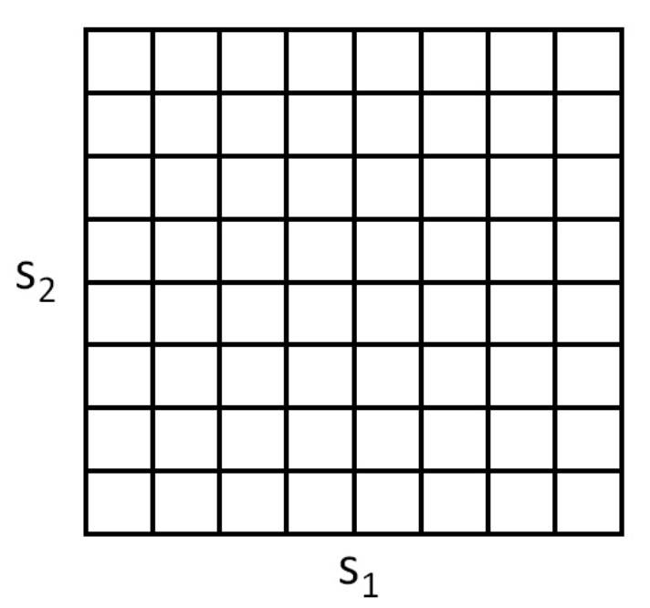
- Here, each grid cell represents a separate discrete state \(\bar{s}\). We can then approximate the continuous-state MDP via a discrete-state one \(\left(\bar{S}, A,\left\{P_{\bar{s} a}\right\}, \gamma, R\right)\) where \(\bar{S}\) is the set of discrete states, \(\left\{P_{\bar{s} a}\right\}\) are our state transition probabilities over the discrete states, and so on. We can then use value iteration or policy iteration to solve for the \(V^{\ast}(\bar{s})\) and \(\pi^{\ast}(\bar{s})\) in the discrete state MDP \(\left(\bar{S}, A,\left\{P_{\bar{s} a}\right\}, \gamma, R\right)\). When our actual system is in some continuous-valued state \(s \in S\) and we need to pick an action to execute, we compute the corresponding discretized state \(\bar{s}\), and execute action \(\pi^{\ast}(\bar{s})\).
- This discretization approach can work well for many problems. However, there are two downsides. First, it uses a fairly naive representation for \(V^{\ast}\) (and \(\left.\pi^{\ast}\right)\). Specifically, it assumes that the value function is takes a constant value over each of the discretization intervals (i.e., that the value function is piecewise constant in each of the gridcells).
- To better understand the limitations of such a representation, consider a supervised learning problem of fitting a function to this dataset:
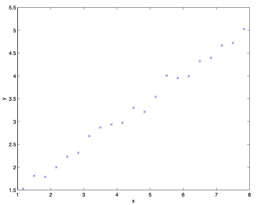
- Clearly, linear regression would do fine on this problem. However, if we instead discretize the \(x\) -axis, and then use a representation that is piecewise constant in each of the discretization intervals, then our fit to the data would look like this:
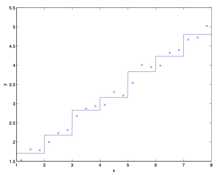
- This piecewise constant representation just isn’t a good representation for many smooth functions. It results in little smoothing over the inputs, and no generalization over the different grid cells. Using this sort of representation, we would also need a very fine discretization (very small grid cells) to get a good approximation.
- A second downside of this representation is called the curse of dimensionality. Suppose \(S=\mathbb{R}^{n}\), and we discretize each of the \(n\) dimensions of the state into \(k\) values. Then the total number of discrete states we have is \(k^{n}\). This grows exponentially quickly in the dimension of the state space \(n\), and thus does not scale well to large problems. For example, with a \(10 \mathrm{D}\) state, if we discretize each state variable into 100 values, we would have \(100^{10}=10^{20}\) discrete states, which is far too many to represent even on a modern desktop computer.
- As a rule of thumb, discretization usually works extremely well for \(1 \mathrm{D}\) and \(2 \mathrm{D}\) problems (and has the advantage of being simple and quick to implement). Perhaps with a little bit of cleverness and some care in choosing the discretization method, it often works well for problems with up to \(4 \mathrm{D}\) states. If you’re extremely clever, and somewhat lucky, you may even get it to work for some \(6 \mathrm{D}\) problems. But it very rarely works for problems any higher dimensional than that.
Value function approximation
- We now describe an alternative method for finding policies in continuous state MDPs, in which we approximate \(V^{\ast}\) directly, without resorting to discretization. This approach, caled value function approximation, has been successfully applied to many RL problems.
Using a model or simulator
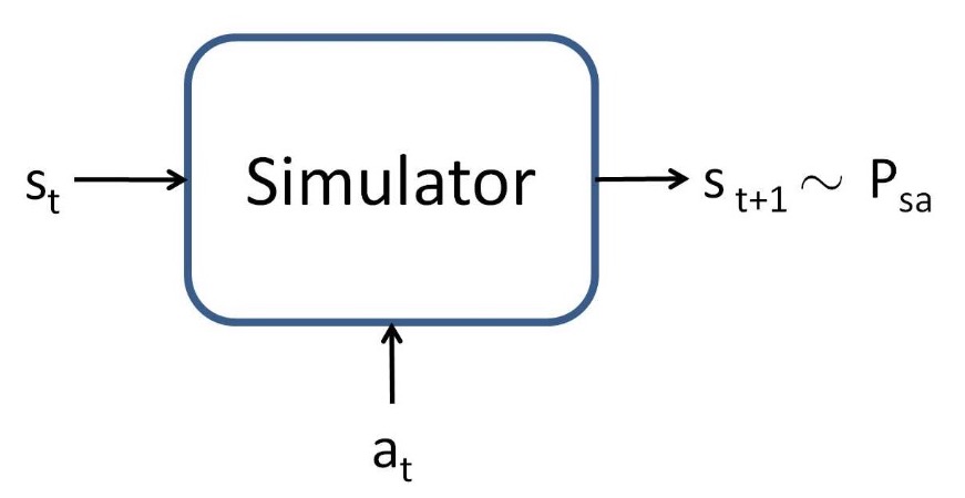
- To develop a value function approximation algorithm, we will assume that we have a model, or simulator, for the MDP. Informally, a simulator is a black-box that takes as input any (continuous-valued) state \(s_{t}\) and action \(a_{t}\), and outputs a next-state \(s_{t+1}\) sampled according to the state transition probabilities \(P_{s_{t} a_{t}}\):
- There are several ways that one can get such a model. One is to use physics simulation. For example, the simulator for the inverted pendulum in \(\mathrm{PS} 4\) was obtained by using the laws of physics to calculate what position and orientation the cart/pole will be in at time \(t+1\), given the current state at time \(t\) and the action \(a\) taken, assuming that we know all the parameters of the system such as the length of the pole, the mass of the pole, and so on. Alternatively, one can also use an off-the-shelf physics simulation software package which takes as input a complete physical description of a mechanical system, the current state \(s_{t}\) and action \(a_{t}\), and computes the state \(s_{t+1}\) of the system a small fraction of a second into the future.
- Open Dynamics Engine is one example of a free/open-source physics simulator that can be used to simulate systems like the inverted pendulum, and that has been a reasonably popular choice among RL researchers.
- An alternative way to get a model is to learn one from data collected in the MDP. For example, suppose we execute \(m\) trials in which we repeatedly take actions in an MDP, each trial for \(T\) timesteps. This can be done picking actions at random, executing some specific policy, or via some other way of choosing actions. We would then observe \(m\) state sequences like the following:
- We can then apply a learning algorithm to predict \(s_{t+1}\) as a function of \(s_{t}\) and \(a_{t}\) For example, one may choose to learn a linear model of the form
- using an algorithm similar to linear regression. Here, the parameters of the model are the matrices \(A\) and \(B\), and we can estimate them using the data collected from our \(m\) trials, by picking
- This corresponds to the maximum likelihood estimate of the parameters.
- Having learned \(A\) and \(B\), one option is to build a deterministic model, in which given an input \(s_{t}\) and \(a_{t}\), the output \(s_{t+1}\) is exactly determined.
-
Specifically, we always compute \(s_{t+1}\) according to Equation \((5)\). Alternatively, we may also build a stochastic model, in which \(s_{t+1}\) is a random function of the inputs, by modelling it as,
\[s_{t+1}=A s_{t}+B a_{t}+\epsilon_{t}\]- where here \(\epsilon_{t}\) is a noise term, usually modeled as \(\epsilon_{t} \sim \mathcal{N}(0, \Sigma)\). (The covariance matrix \(\Sigma\) can also be estimated from data in a straightforward way.)
- Here, we’ve written the next-state \(s_{t+1}\) as a linear function of the current state and action; but of course, non-linear functions are also possible. Specifically, one can learn a model \(s_{t+1}=A \phi_{s}\left(s_{t}\right)+B \phi_{a}\left(a_{t}\right)\), where \(\phi_{s}\) and \(\phi_{a}\) are some non-linear feature mappings of the states and actions. Alternatively, one can also use non-linear learning algorithms, such as locally weighted linear regression, to learn to estimate \(s_{t+1}\) as a function of \(s_{t}\) and \(a_{t}\). These approaches can also be used to build either deterministic or stochastic simulators of an MDP.
Fitted value iteration
- We now describe the fitted value iteration algorithm for approximating the value function of a continuous state MDP. In the sequel, we will assume that the problem has a continuous state space \(S=\mathbb{R}^{n}\), but that the action space \(A\) is small and discrete.
- In practice, most MDPs have much smaller action spaces than state spaces. E.g., a car has a \(6 \mathrm{D}\) state space, and a \(2 \mathrm{D}\) action space (steering and velocity controls); the inverted pendulum has a \(4 \mathrm{D}\) state space, and a \(1 \mathrm{D}\) action space; a helicopter has a \(12 \mathrm{D}\) state space, and a \(4 \mathrm{D}\) action space. So, discretizing ths set of actions is usually less of a problem than discretizing the state space would have been.
- Recall that in value iteration, we would like to perform the update:
- In our section on value iteration and policy iteration, we had written the value iteration update with a summation rather than an integral over states:
- Note that the new notation reflects that we are now working in continuous states rather than discrete states.
- The main idea of fitted value iteration is that we are going to approximately carry out this step, over a finite sample of states \(s^{(1)}, \ldots, s^{(m)}\). Specifically, we will use a supervised learning algorithm-linear regression in our description below - to approximate the value function as a linear or non-linear function of the states:
- Here, \(\phi\) is some appropriate feature mapping of the states.
- For each state \(s\) in our finite sample of \(m\) states, fitted value iteration will first compute a quantity \(y^{(i)}\), which will be our approximation to:
- Note that this is the right hand side of Equation \((7)\).
- Then, it will apply a supervised learning algorithm to try to get \(V(s)\) close to:
-
or, in other words, to try to get \(V(s)\) close to \(\left(y^{(i)}\right)\).
- In detail, the algorithm is as follows:
- Randomly sample \(m\) states \(s^{(1)}, s^{(2)}, \ldots s^{(m)} \in S\).
- Initialize \(\theta:=0\).
- Repeat
- For \(i=1, \ldots, m\)
- For each action \(a \in A\)
- Sample \(s_{1}^{\prime}, \ldots, s_{k}^{\prime} \sim P_{s^{(i)} a}\) (using a model of the MDP).
- Set \(q(a)=\frac{1}{k} \sum_{j=1}^{k} R\left(s^{(i)}\right)+\gamma V\left(s_{j}^{\prime}\right)\).
- \(//\) Hence, \(q(a)\) is an estimate of: \(R\left(s^{(i)}\right)+\gamma \mathrm{E}_{s^{\prime} \sim P_{s}(i)_{a}}\left[V\left(s^{\prime}\right)\right]\)
- Set \(y^{(i)}=\max _{a} q(a)\)
- \(//\) Hence, \(y^{(i)}\) is an estimate of:
\(R\left(s^{(i)}\right)+\gamma \max _{a} \mathrm{E}_{s^{\prime} \sim P_{s}(i)_{a}}\left[V\left(s^{\prime}\right)\right]\)
- \(//\) In the original value iteration algorithm (over discrete states) we updated the value function according to \(V\left(s^{(i)}\right):=y^{(i)}\). In this algorithm, we want \(V\left(s^{(i)}\right) \approx y^{(i)}\), which we’ll achieve using supervised learning (linear regression).
- \(//\) Hence, \(y^{(i)}\) is an estimate of:
\(R\left(s^{(i)}\right)+\gamma \max _{a} \mathrm{E}_{s^{\prime} \sim P_{s}(i)_{a}}\left[V\left(s^{\prime}\right)\right]\)
- For each action \(a \in A\)
- Set:
- For \(i=1, \ldots, m\)
- Above, we had written out fitted value iteration using linear regression as the algorithm to try to make \(V\left(s^{(i)}\right)\) close to \(y^{(i)}\). That step of the algorithm is completely analogous to a standard supervised learning (regression) problem in which we have a training set \(\left(x^{(1)}, y^{(1)}\right),\left(x^{(2)}, y^{(2)}\right), \ldots,\left(x^{(m)}, y^{(m)}\right)\), and want to learn a function mapping from \(x\) to \(y\); the only difference is that here \(s\) plays the role of \(x\). Even though our description above used linear regression, clearly other regression algorithms (such as locally weighted linear regression) can also be used.
- Unlike value iteration over a discrete set of states, fitted value iteration cannot be proved to always to converge. However, in practice, it often does converge (or approximately converge), and works well for many problems. Note also that if we are using a deterministic simulator/model of the MDP, then fitted value iteration can be simplified by setting \(k=1\) in the algorithm. This is because the expectation in Equation \((7)\) becomes an expectation over a deterministic distribution, and so a single example is sufficient to exactly compute that expectation. Otherwise, in the algorithm above, we had to draw \(k\) samples, and average to try to approximate that expectation (see the definition of \(q(a)\), in the algorithm pseudo-code).
- Finally, fitted value iteration outputs \(V\), which is an approximation to \(V^{\ast}\). This implicitly defines our policy. Specifically, when our system is in some state \(s\), and we need to choose an action, we would like to choose the action:
- The process for computing/approximating this is similar to the inner-loop of fitted value iteration, where for each action, we sample \(s_{1}^{\prime}, \ldots, s_{k}^{\prime} \sim P_{s a}\) to approximate the expectation. (And again, if the simulator is deterministic, we can set \(k=1\).)
- In practice, there’re often other ways to approximate this step as well. For example, one very common case is if the simulator is of the form \(s_{t+1}=\) \(f\left(s_{t}, a_{t}\right)+\epsilon_{t}\), where \(f\) is some determinstic function of the states (such as \(\left.f\left(s_{t}, a_{t}\right)=A s_{t}+B a_{t}\right)\), and \(\epsilon\) is zero-mean Gaussian noise. In this case, we can pick the action given by,
-
In other words, here we are just setting \(\epsilon_{t}=0\) (i.e., ignoring the noise in the simulator), and setting \(k=1\). Equivalently, this can be derived from Equation \((8)\) using the approximation,
\[\mathrm{E}_{s^{\prime}}\left[V\left(s^{\prime}\right)\right] \approx V\left(\mathrm{E}_{s^{\prime}}\left[s^{\prime}\right]\right) \tag{9}\] \[=V(f(s, a)) \tag{10}\]- where the expection is over the random \(s^{\prime} \sim P_{s a}\). So long as the noise terms \(\epsilon_{t}\) are small, this will usually be a reasonable approximation.
-
However, for problems that don’t lend themselves to such approximations, having to sample \(k|A|\) states using the model, in order to approximate the expectation above, can be computationally expensive.
References
Citation
If you found our work useful, please cite it as:
@article{Chadha2020DistilledReinforcementLearningandAdaptiveControl,
  title   = {Reinforcement Learning and Adaptive Control},
  author  = {Chadha, Aman},
  journal = {Distilled Notes for Stanford CS229: Machine Learning},
  year    = {2020},
  note    = {\url{https://aman.ai}}
}