CS229 • Newton's method
Newton’s method
Overview
- Gradient ascent is a very effective algorithm, but it takes baby steps at every single iteration and thus needs a lot of iterations to converge.
- Newton’s method is another algorithm for maximizing \(\ell(\theta)\) which allows you to take much bigger steps and thus converge much earlier than gradient ascent, with usually an order of magnitude lesser number of iterations. However, each iteration tends to be more expensive in this case.
- To get started, let’s consider Newton’s method for finding a zero of a function. Let’s assume that this is a function of a one-dimensional/scalar parameter \(\theta\). Specifically, suppose we have a function \(f: \mathbb{R} \mapsto \mathbb{R}\), and we wish to find a value of \(\theta\) such that \(f(\theta)=0\). Here, \(\theta \in \mathbb{R}\) is a real number. As such, the update rule for Newton’s method is given by,
- We shall derive the above equation with the help of our graphical explanation of Newton’s method in the section on update rule below.
- This method has a natural interpretation in which we can think of it as approximating the function \(f(\cdot)\) via a linear function that is tangent to \(f(\cdot)\) at the current value of \(\theta\). Solving for where that linear function equals to 0, yields the updated value of \(\theta\).
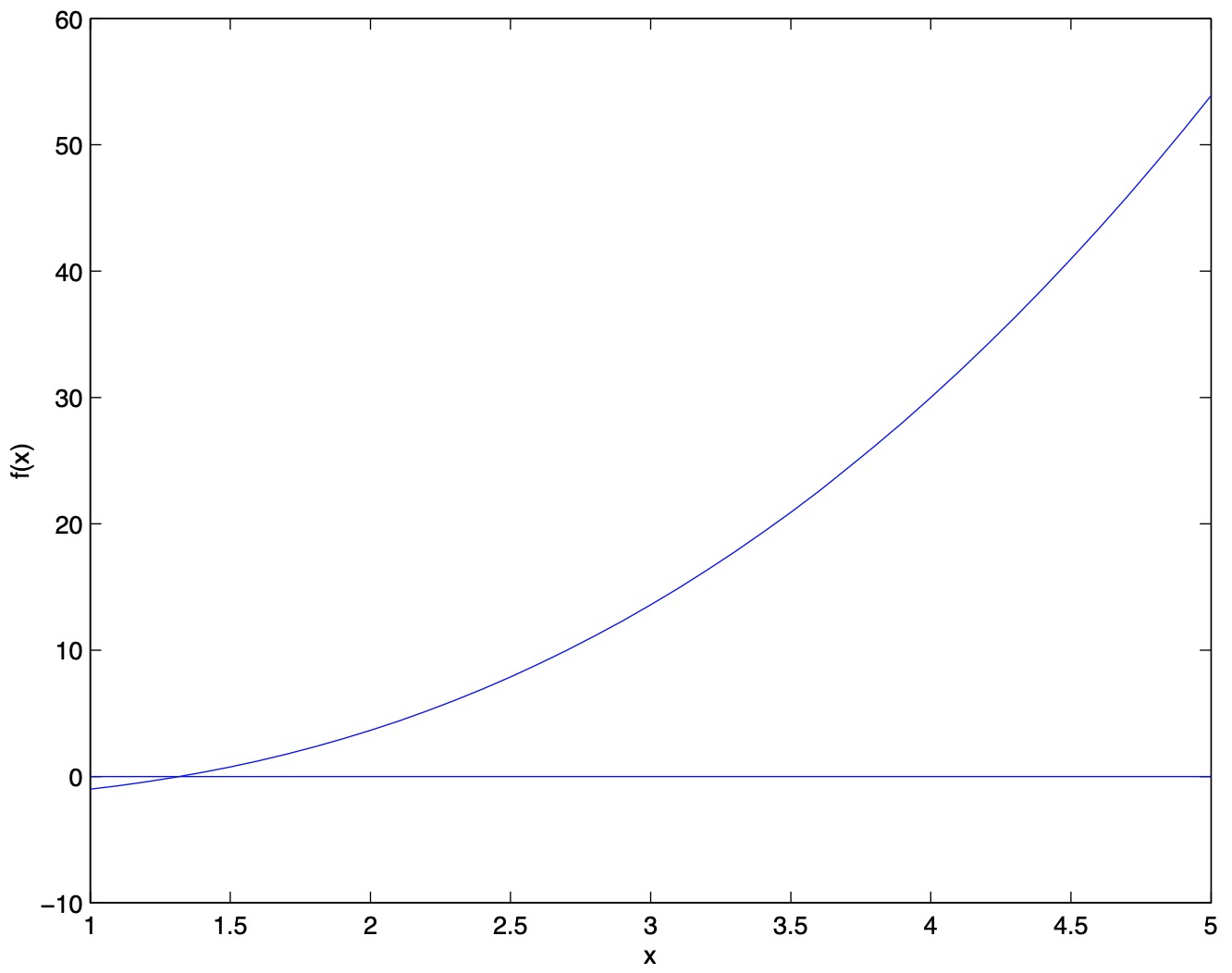
- Let’s visualize Newton’s method in action. In the below graph, we see the function \(f(\cdot)\) plotted along with the line \(y=0\). We’re trying to find \(\theta\) such that \(f(\theta)=0\). The value of \(\theta\) that achieves this is \(\approx\) 1.3.
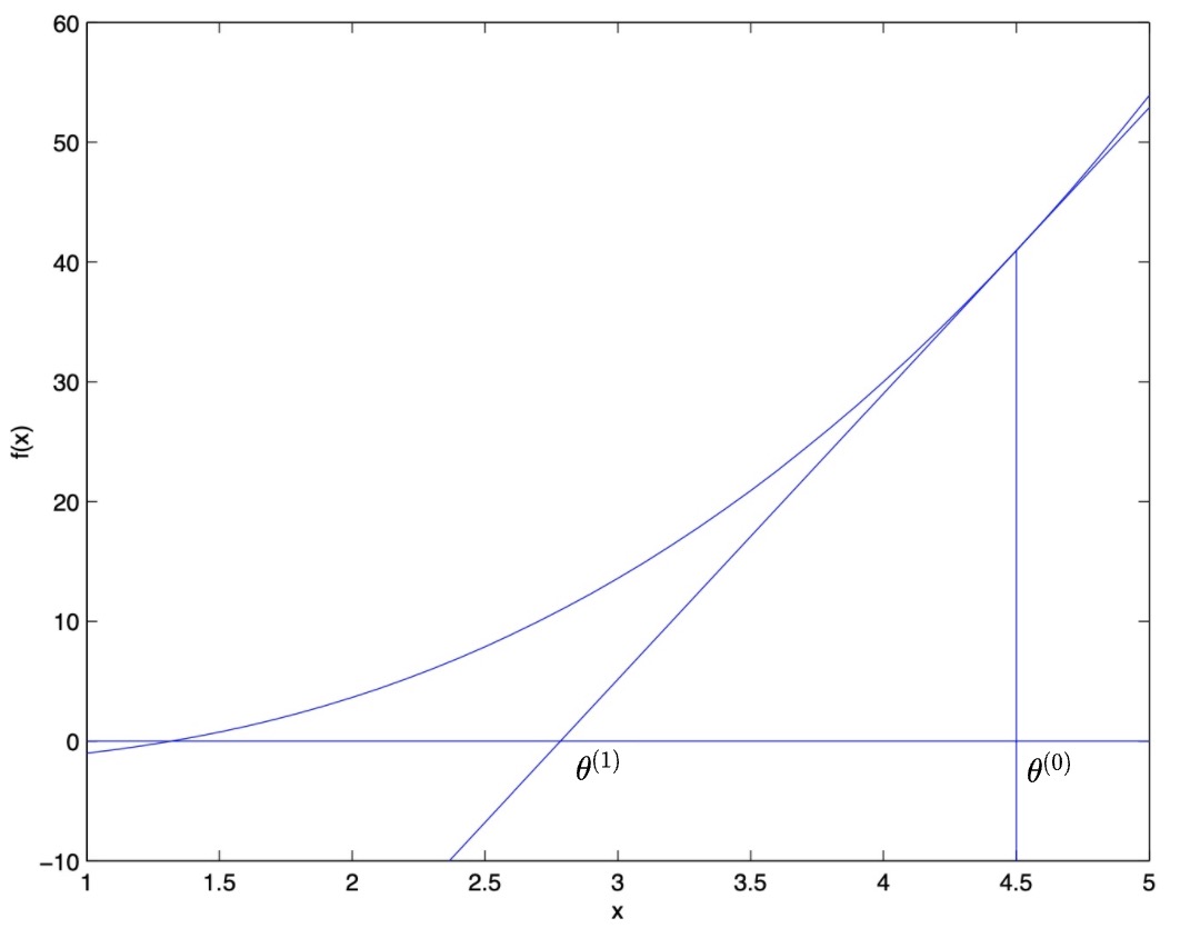
- Suppose we initialized the algorithm with \(\theta=4.5\). Let this initial value of \(\theta\) be denoted by \(\theta^{(0)}\). Newton’s method fits a straight line tangent to \(f(\cdot)\) at \(\theta=4.5\), and uses straight line approximation to \(f(\cdot)\) to solve for where \(f(\cdot)\) touches the horizontal axis (i.e., we’re looking for the x-intercept of the line, which can be found by setting \(y = 0\)). This give us the next guess for \(\theta\), denoted by \(\theta^{(1)}\), which is \(\approx\) 2.8 (cf. graph below).
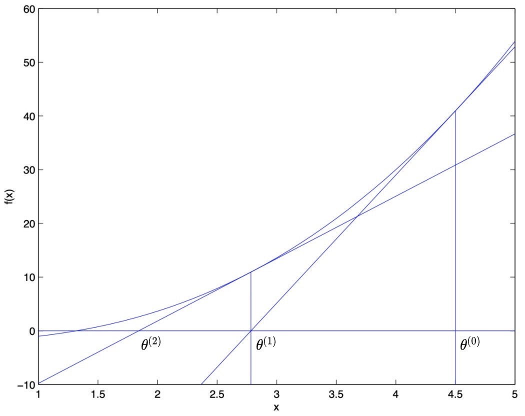
- The graph below shows the result of another iteration, which updates \(\theta\) to \(\theta^{(2)}\) which is \(\approx\) 1.8. After a few more iterations, we rapidly approach \(\theta=1.3\).
- Newton’s method gives a way of getting to \(f(\theta)=0\). What if we want to use it to maximize the log likelihood function \(\ell(\cdot)\)? The maxima of \(\ell(\theta)\) corresponds to points where its first derivative \(\ell^{\prime}(\theta)\) is 0. So, by letting \(f(\theta)=\ell^{\prime}(\theta)\), we can use the same algorithm to maximize \(\ell(\cdot)\), and we obtain the following update rule:
- Generalizing the above equation in terms of indices \(t\) and \(t+1\), the update rule for \(\theta^{(t+1)}\) is given by difference between \(\theta^{(t)}\) and the first derivative of \(\ell(\cdot)\) divided by the second derivative of \(\ell(\cdot)\):
- Note that if we wish to minimize a function, rather than maximize it, we still need to find a point where its first derivative \(\ell^{\prime}(\theta)\) is 0.
Update rule
- Let’s derive the update rule for Newton’s method graphically. Refer the graph below based on the example we looked at in the above section on Newton’s method overview.
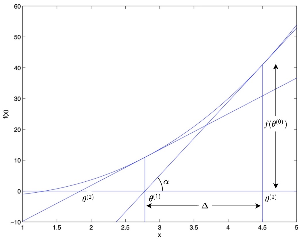
- From the graph,
- The slope of the line having an angle \(\alpha\) with the horizontal is:
- Recall that the first derivative of a function at a particular point represents the slope of the tangent to the function at that point. Thus,
- Rearranging the above equation to get the value of \(\Delta\),
- Plugging in the value of \(\Delta\) in the equation for \(\theta^{(1)}\) gives us the update rule for Newton’s method,
- Generally speaking, the update rule governs the process of going from \(\theta^{(t)}\) to \(\theta^{(t+1)}\). Generalizing the above equation in terms of indices \(t\) and \(t+1\),
Quadratic convergence
- Newton’s method enjoys a property called quadratic convergence.
- An informal explanation of what this implies is as follows. Assume that on one iteration Newton’s method has 0.01 error (i.e., on the X-axis, you’re 0.01 away from the from the true minimum or where \(f’(\cdot)\) is equal to 0). After the iteration, the error could quadratically jump to 0.0001, and after two iterations it can further jump to 0.00000001.
- Thus, the iterations in Newton’s method represent quadratic steps, and the number of significant digits that you have converged to the minimum, double on a single iteration.
- One way to interpret this is as follows: after a single iteration, Newton’s method becomes accurate, after another iteration it becomes much more accurate, and so on. And so when you get near the minimum, Newton’s method converges extremely rapidly compared to gradient descent. This is essentially why Newton’s method requires relatively few iterations.
Newton’s method for vectors
-
In our logistic regression setting, \(\theta\) is vector-valued, so we need to generalize Newton’s method from a single-dimensional to a multi-dimensional case. The generalization of Newton’s method to a multi-dimensional setting (also called the Newton-Raphson method) is given by,
\[\theta:=\theta-H^{-1} \nabla_{\theta} \ell(\theta)\]- where,
- \(\nabla_{\theta} \ell(\theta)\) is the vector of partial derivatives of \(\ell(\theta)\) with respect to the \(\theta_{i}\)’s.
- \(H\) is an \(n \times n\) matrix (actually, \((n+1) \times (n+1)\), assuming that we include the intercept term) called the Hessian. The Hessian thus becomes a squared matrix \(\mathbb{R}^{(n+1) \times (n+1)}\) where the \((n+1)\) dimension is equal to the size of the parameter vector \(\theta\).
- where,
-
The Hessian matrix is defined as the matrix of second-order partial derivatives whose entries are given by,
- As seen in the section on quadratic convergence, Newton’s method typically enjoys faster convergence than (batch) gradient descent, and requires fewer iterations to get very close to the minimum. However, in case of very high-dimensional problems, where \(\theta\) is a high-dimensional vector, each iteration/step of Newton’s can, however, be more expensive than one iteration of gradient descent, since it requires finding and inverting an \(n \times n\) Hessian; but so long as \(n\) is not too large, it is usually much faster overall.
- If \(\theta\) is 10-dimensional, this involves inverting a \(10 \times 10\) matrix, which is tractable.
- If \(\theta\) is 100,000-dimensional, each iteration of Newton’s method would require computing a \(100,000 \times 100,000\) matrix and inverting that, which is very compute intensive.
- Rules of thumb
- Use Newton’s method if you have a small number of parameters (i.e., where the computational cost per iteration is manageable), say 10 - 50 parameters because you’ll converge in \(\sim\) 10 - 15 iterations.
- Use gradient descent if you have a very large number of parameters, say 10,000 parameters. The computation cost with Newton’s method in dealing with a \(10,000 \times 10,000\) matrix tends to be prohibitive.
- As an aside, when Newton’s method is applied to maximize the logistic regression log likelihood function \(\ell(\theta)\), the resulting method is also called Fisher scoring.
Further reading
Here are some (optional) links you may find interesting for further reading:
- Intercepts of lines delves into x and y intercepts of a line and how you can obtain them.
References
Citation
If you found our work useful, please cite it as:
@article{Chadha2020DistilledNewtonMethod,
  title   = {Newton's method},
  author  = {Chadha, Aman},
  journal = {Distilled Notes for Stanford CS229: Machine Learning},
  year    = {2020},
  note    = {\url{https://aman.ai}}
}