CS229 • Logistic Regression
The classification problem
- Let’s now take the framework we’ve developed so far and apply it to a different type of problem, the classification problem. This is just like the regression problem, except that the values \(y\) we now want to predict take on only a small number of discrete values.
- For now, we will focus on the binary classification problem in which \(y\) can take on only two values, i.e., \(y \in {0, 1}\). Note that most of the observations we’ll make here and the conclusions that we’ll reach will also generalize to the multi-class case. For instance, if we are trying to build a spam classifier for email, \(x^{(i)}\) may be a vector of features for an email, and \(y^{(i)}\) may be 1 if it is spam mail, and 0 otherwise. 0 is also called the negative class, and 1 the positive class, and they are sometimes also denoted by the symbols \(“-“\) and \(“+”\). Given \(x^{(i)}\), the corresponding \(y^{(i)}\) is also called the label for the training example.
Motivation
- We could approach the classification problem ignoring the fact that \(y\) is discrete-valued, and use the linear regression algorithm to predict \(y\) given \(x\).
- Let’s try applying linear regression to a binary classification dataset for a spam classifier. Just fit a straight line through data and then take the straight line and threshold it at 0.5, and then apply a threshold of 0.5. A value beyond 0.5 gets rounded off to 1, and if it’s below 0.5, round it off to 0.
- However, it is easy to construct examples where this method performs very poorly. For some datasets, it can be really obvious what the pattern is, and the decision boundary seems more or less clear. But let’s say we now update the dataset to just add an additional example which is an outlier. If you fit a straight line through this new dataset with the new datapoint, you end up with a very different decision boundary after the thresholding operation.
- Thus, while in some simplistic cases, using linear regression for classification does pan out well, generally linear regression is not a good algorithm for classification.
- Also, intuitively, it sounds unnatural for \(h_{\theta}(x)\) to take on values \(\ll\,0\) and \(\gg\,1\), when we know that \(y \in {0, 1}\).
Logistic regression
- Logistic regression is one of the most commonly used classification algorithms.
-
As we design the logistic regression algorithm, one of the things we might naturally want is for the hypothesis \(h_{\theta}(x)\) to output values \(\in \{0, 1\}\). To that end, let’s choose our hypotheses \(h_{\theta}(x)\) as:
\[h_{\theta}(x)=g(\theta^{T} x)=\frac{1}{1+e^{-\theta^{T} x}}\]- where \(g(z)=\frac{1}{1+e^{-z}}\) is called the logistic function or the sigmoid function.
- Since \(\theta^{T} x\) could be \(\ll\,0\) and \(\gg\,1\), which is not very natural for a binary classification problem with labels \(\in \{0, 1\}\), logistic regression passes it through the sigmoid function \(g(z)\) which forces/squashes/compresses/squeezes/collapses the input from \(\in [-\infty, \infty]\) to an output \(\in [0, 1]\).
- Given the output is within permissible range of probability values, i.e., \([0, 1]\), it can be interpreted as a probability measure.
- Here is a plot showing \(g(z)\):
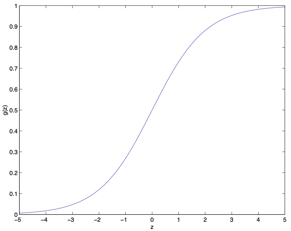
- As shown in the plot above, \(g(z)\) starts off really close to 0, then rises and asymptotes towards 1. In other words, \(g(z) \rightarrow 1\) as \(z \rightarrow \infty\), and \(g(z) \rightarrow 0\) as \(z \rightarrow −\infty\). Note that \(g(z) = 0.5\), i.e., it has a y-intercept of (i.e., it cuts the x-axis at) \(0.5\).
- Moreover, \(g(z)\), and hence also \(h_{\theta}(x)\), are always bounded \(\in [0, 1]\). As before, we are keeping the convention of letting \(x_0 = 1\), so that \(\theta^T x = \theta_0 + \sum_{j=1}^n \theta_j x_j\).
- For now, let’s take the choice of \(g(\cdot)\) as given. Other functions that smoothly increase from 0 to 1 can also be used, but for a couple of reasons that we’ll see later (when we discuss generative learning models and generative learning algorithms), the choice of the logistic function is a fairly natural one. Before moving on, here’s how we compute the derivative of the sigmoid function, which we write as \(g’(\cdot)\):
- For a more detailed derivation of the derivative of the sigmoid function, refer our primer on the derivative of the sigmoid function.
Update rule
- So, given the logistic regression model, how do we fit \(\theta\) for it? Following the derivation for least squares regression using the maximum likelihood estimator under a set of assumptions, let’s endow our classification model with a set of probabilistic assumptions, and then fit the parameters via maximum likelihood.
- Because \(y\) can be 0 or 1, the probabilities \(P(y^{(i)}=0 \mid x^{(i)} ; \theta)\) and \(P(y^{(i)}=1 \mid x^{(i)} ; \theta)\) are complementary and thus add up to 1. Thus, for a single training example \((x^{(i)}, y^{(i)})\),
- This can be written more compactly as a single equation as follows:
- Note that the above is just a nifty way to take the equations for \(P(y^{(i)}=0 \mid x^{(i)} ; \theta)\) and \(P(y^{(i)}=1 \mid x^{(i)} ; \theta)\) and compress them into one equation with a little exponentiation trick. Depending on whether y is 0 or 1, one of these two terms switches off, because it’s exponentiated to the power of 0, and anything to the power of 0 is just equal to 1. This leaves us with the other term and thus selects the appropriate equation.
- If \(y = 0\), the equation for \(P(y^{(i)} \mid x^{(i)})\) transforms to:
- If \(y = 1\), the equation for \(P(y^{(i)} \mid x^{(i)})\) transforms to:
- Assuming that the \(m\) training examples were generated independently, we can write down the likelihood of the parameters \(L(\theta)\) as:
- As before, it’s easier to maximize the log likelihood rather than the likelihood:
-
Next, per maximum likelihood estimation, we’ll need to find the value of \(\theta\) that maximizes \(\ell(\theta)\). Similar to our derivation in the case of linear regression, the algorithm we’re going to use to choose \(\theta\) to maximize the log-likelihood is (batch) gradient ascent. Our update rule is thus given by,
\[\theta:=\theta+\alpha \nabla_{\theta} \ell(\theta)\]- where \(\alpha\) is the learning rate (i.e., the step size).
- Note that there’s two differences in our update rule in the case of logistic regression vs. linear regression:
- Instead of the squared cost function \(J(\theta)\), you’re trying to optimize the log-likelihood \(\ell(\theta)\).
- The positive rather than negative sign in the update rule formula, indicating that we’re performing gradient ascent rather than descent, since we’re maximizing, rather than minimizing the function.
- In particular, taking a deeper look at the update rule for \(\theta\) in case of linear regression, because we sought to minimize the squared error by carrying out gradient descent, we had a minus sign. With logistic regression, since we’re trying to maximize the log likelihood by by carrying out gradient ascent, there’s a plus sign.
- A graphical interpretation of this is that gradient descent is trying to climb down a hill represented by a convex function, whereas gradient ascent is trying to climb up a hill represented by a concave function.
- Let’s plug in the formula for \(h(x^{(i)})\), and take derivatives to derive the stochastic gradient ascent rule:
-
Above, we used the fact that \(g^{\prime}(z) = g(z)(1-g(z))\). This therefore gives us the stochastic gradient ascent rule:
\[\theta_{j}:=\theta_{j}+\alpha\left(y^{(i)}-h_{\theta}(x^{(i)})\right) x_{j}^{(i)}\]- where \(\alpha\) is the learning rate and \(x_{j}^{(i)}\) represents the the \(j^{th}\) feature of the \(i^{th}\) training sample.
-
Note that the above equation represents the update rule for a single training example \((x^{(i)}, y^{(i)})\). Generalizing this for the entire training set of \(m\) examples,
- If we compare this to the LMS update rule, we see that it looks identical; but this is not the same algorithm, because \(h_{\theta}(x^{(i)})\) is now defined as a non-linear function of \(\theta^{T} x^{(i)}\). Nonetheless, it might be a little surprising that we end up with the same update rule for a rather different algorithm and learning problem. This is actually not a coincidence, and is infact a general property of a much bigger class of algorithms called generalized linear models.
Citation
If you found our work useful, please cite it as:
@article{Chadha2020DistilledLogisticRegression,
  title   = {Logistic Regression},
  author  = {Chadha, Aman},
  journal = {Distilled Notes for Stanford CS229: Machine Learning},
  year    = {2020},
  note    = {\url{https://aman.ai}}
}