CS229 • Ensemble Methods
Overview
-
We now cover methods by which we can aggregate the output of trained models. We will use Bias-Variance analysis as well as the example of decision trees to probe some of the trade-offs of each of these methods.
-
To understand why we can derive benefit from ensembling, let us first recall some basic probability theory. Say we have \(n\) independent, identically distributed (i.i.d.) random variables \(X_{i}\) for \(0 \leq i<n\). Assume \(\operatorname{Var}\left(X_{i}\right)=\sigma^{2}\) for all \(X_{i}\). Then we have that the variance of the mean is:
- Now, if we drop the independence assumption (so the variables are only i.d.), and instead say that the \(X_{i}\)’s are correlated by a factor \(\rho\), we can show that:
- Where in Step 3 we use the definition of pearson correlation coefficient,
- Now, if we consider each random variable to be the error of a given model, we can see that both increasing the number of models used (causing the second term to vanish) as well as decreasing the correlation between models (causing the first term to vanish and returning us to the i.i.d. definition) leads to an overall decrease in variance of the error of the ensemble.
- There are several ways by which we can generate de-correlated models, including:
- Using different algorithms
- Using different training sets
- Bagging
- Boosting
- While the first two are fairly straightforward, they involve large amounts of additional work. In the following sections, we will cover the latter two techniques, boosting and bagging, as well as their specific uses in the context of decision trees.
Bagging
Boostrap
- Bagging stands for “Boostrap Aggregation” and is a variance reduction ensembling method. Bootstrap is a method from statistics traditionally used to measure uncertainty of some estimator (e.g. mean).
- Say we have a true population \(P\) that we wish to compute an estimator for, as well a training set \(S\) sampled from \(P(S \sim P)\). While we can find an approximation by computing the estimator on \(S\), we cannot know what the error is with respect to the true value. To do so we would need multiple independent training sets \(S_{1}, S_{2}, \ldots\) all sampled from \(P\).
- However, if we make the assumption that \(S=P\), we can generate a new bootstrap set \(Z\) sampled with replacement from \(S(Z \sim S,|Z|=|S|)\). In fact we can generate many such samples \(Z_{1}, Z_{2}, \ldots, Z_{M}\). We can then look at the variability of our estimate across these bootstrap sets to obtain a measure of error.
Aggregation
- Now, returning to ensembling, we can take each \(Z_m\) and train a machine learning model \(G_m\) on each, and define a new aggregate predictor:
- This process is called bagging. Referring back to equation \((4)\), we have that the variance of \(M\) correlated predictors is:
- Bagging creates less correlated predictors than if they were all simply trained on \(S\), thereby decreasing \(\rho\). While the bias of each individual predictor increases due to each bootstrap set not having the full training set available, in practice it has been found that the decrease in variance outweighs the increase in bias. Also note that increasing the number of predictors \(M\) can’t lead to additional overfitting, as \(\rho\) is insensitive to \(M\) and therefore overall variance can only decrease.
- An additional advantage of bagging is called out-of-bag estimation. It can be shown that each bootstrapped sample only contains approximately \(\frac{2}{3}\) of \(S\), and thus we can use the other \(\frac{1}{3}\) as an estimate of error, called outof-bag error. In the limit, as \(M \rightarrow \infty\), out-of-bag error gives an equivalent result to leave-one-out cross-validation.
Bagging + Decision Trees
- Recall that fully-grown decision trees are high variance, low bias models, and therefore the variance-reducing effects of bagging work well in conjunction with them. Bagging also allows for handling of missing features: if a feature is missing, exclude trees in the ensemble that use that feature in our of their splits. Though if certain features are particularly powerful predictors they may still be included in most if not all trees.
- A downside to bagged trees is that we lose the interpretability inherent in the single decision tree. One method by which to re-gain some amount of insight is through a technique called variable importance measure. For each feature, find each split that uses it in the ensemble and average the decrease in loss across all such splits. Note that this is not the same as measuring how much performance would degrade if we did not have this feature, as other features might be correlated and could substitute.
- A final but important aspect of bagged decision trees to cover is the method of random forests. If our dataset contained one very strong predictor, then our bagged trees would always use that feature in their splits and end up correlated. With random forests, we instead only allow a subset of features to be used at each split. By doing so, we achieve a decrease in correlation \(\rho\) which leads to a decrease in variance. Again, there is also an increase in bias due to the restriction of the feature space, but as with vanilla bagged decision trees this proves to not often be an issue.
- Finally, even powerful predictors will no longer be present in every tree (assuming sufficient number of trees and sufficient restriction of features at each split), allowing for more graceful handling of missing predictors.
Key takeaways
- To summarize, some of the primary benefits of bagging, in the context of decision trees, are:
- Decrease in variance (even more so for random forests)
- Better accuracy
- Free validation set
- Support for missing values
- While some of the disadvantages include:
- Incrase in bias (even more so for random forests)
- Harder to interpret
- Still not additive
- More expensive
Boosting
Intuition
- Bagging is a variance-reducing technique, whereas boosting is used for bias reduction. We therefore want high bias, low variance models, also known as weak learners. Continuing our exploration via the use of decision trees, we can make them into weak learners by allowing each tree to only make one decision before making a prediction; these are known as decision stumps.
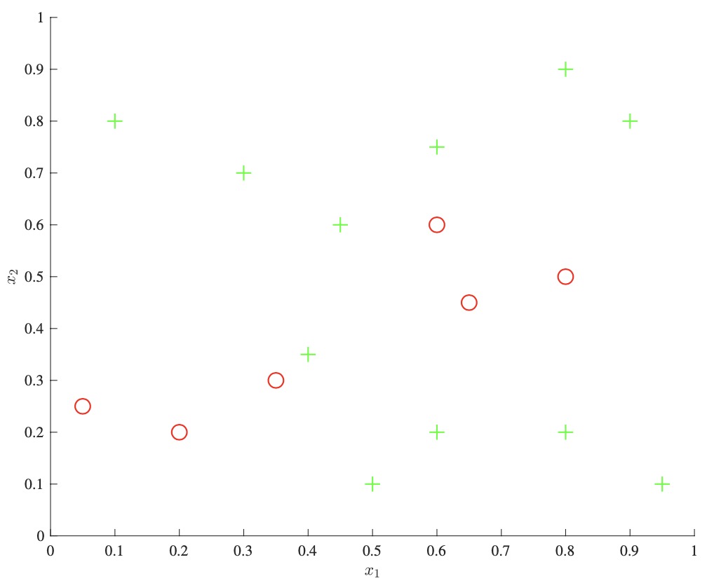
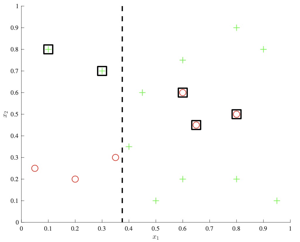
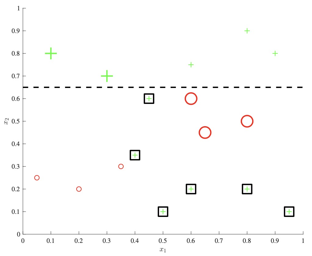
- We explore the intuition behind boosting via the example above. We start with a dataset on the left, and allow a single decision stump to be trained, as seen in the middle panel. The key idea is that we then track which examples the classifier got wrong, and increase their relative weight compared to the correctly classified examples. We then train a new decision stump which will be more incentivized to correctly classify these “hard negatives.” We continue as such, incrementally re-weighting examples at each step, and at the end we output a combination of these weak learners as an ensemble classifier.
Adaboost
-
Having covered the intuition, let us look at one of the most popular boosting algorithms, Adaboost, reproduced below:
- Algorithm 0: Adaboost
- Input: Labeled training data \(\left(x_{1}, y_{1}\right),\left(x_{2}, y_{2}\right), \ldots\left(x_N, y_N\right)\)
- Output: Ensemble classifer \(f(x)\)
- \(w_i \leftarrow \frac{1}{N}\) for \(i=1,2 \ldots, N\).
- for \(m=0\) to \(M\) do
- Fit weak classifier \(G_m\) to training data weighted by \(w_i\)
- Compute weighted error \(\operatorname{err}_m=\frac{\sum_{i} w_i \mathbb{1}\left(y_i \neq G_m\left(x_i\right)\right)}{\sum w_i}\)
- Compute weight \(\alpha_m=\log \left(\frac{1-e r r_m}{\operatorname{err} m}\right)\)
- \(w_i \leftarrow w_i * \exp \left(\alpha_m \mathbb{1}\left(y_{i} \neq G_m\left(x_{i}\right)\right)\right)\)
- end
- \(f(x)=\operatorname{sign}\left(\sum_m \alpha_m G_m(x)\right)\)
- The weightings for each example begin out even, with misclassified examples being further up-weighted at each step, in a cumulative fashion. The final aggregate classifier is a summation of all the weak learners, weighted by the negative log-odds of the weighted error.
- We can also see that due to the final summation, this ensembling method allows for modeling of additive terms, increasing the overall modeling capability (and variance) of the final model. Each new weak learner is no longer independent of the previous models in the sequence, meaning that increasing \(M\) leads to an increase in the risk of overfitting.
- The exact weightings used for Adaboost appear to be somewhat arbitrary at first glance, but can be shown to be well justified. We shall approach this in the next section through a more general framework of which Adaboost is a special case.
Forward Stagewise Additive Modeling
-
The Forward Stagewise Additive Modeling algorithm reproduced below is a framework for ensembling:
- Algorithm 1: Forward Stagewise Additive Modeling
- Input: Labeled training data \(\left(x_{1}, y_{1}\right),\left(x_{2}, y_{2}\right), \ldots\left(x_N, y_N\right)\)
- Output: Ensemble - classifer \(f(x)\)
- Initialize \(f_0(x)=0\)
- for \(m=0\) to \(M\) do
- Compute \(\left(\beta_m, \gamma_m\right)=\operatorname*{arg\,min}_{\beta, \gamma} \sum_{i=1}^N L\left(y_{i}, f_{m-1}\left(x_{i}\right)+\beta G\left(x_{i} ; - \gamma\right)\right)\)
- Set \(f_m(x)=f_{m-1}(x)+\beta_m G\left(x ; y_{i}\right)\)
- end
- \(f(x)=f_m(x)\)
- Close inspection reveals that few assumptions are made about the learning problem at hand, the only major ones being the additive nature of the ensembling as well as the fixing of all previous weightings and parameters after a given step. We again have weak classifiers \(G(x)\), though this time we explicitly parameterize them by their parameters \(\gamma\). At each step we are trying to find the next weak learner’s parameters and weighting so to best match the remaining error of the current ensemble.
- As a concrete implementation of this algorithm, using a squared loss would be the same as fitting individual classifiers to the residual \(y_{i}-f_{m-1}\left(x_{i}\right)\). Furthermore, it can be shown that Adaboost is a special case of this formulation, specifically for 2-class classification and exponential loss:
- For further details regarding the connection between Adaboost and Forward Stagewise Additive Modeling, the interested reader is referred to chapter 10.4 Exponential Loss and AdaBoost in Elements of Statistical Learning.
Gradient Boosting
- In general, it is not always easy to write out a closed-form solution to the minimization problem presented in Forward Stagewise Additive Modeling. High-performing methods such as xgoost resolve this issue by turning to numerical optimization.
- One of the most obvious things to do in this case would be to take the derivative of the loss and perform gradient descent. However, the complication is that we are restricted to taking steps in our model class - we can only add in parameterized weak learners \(G(x, \gamma)\), not make arbitrary moves in the input space.
- In gradient boosting, we instead compute the gradient at each training point with respect to the current predictor (typically a decision stump):
- We then train a new regression predictor to match this gradient and use it as the gradient step. In Forward Stagewise Additive Modeling, this works out to:
Key takeaways
- To summarize, some of the primary benefits of boosting are:
- Decrease in bias
- Better accuracy
- Additive modeling
- While some of the disadvantages include:
- Increase in variance
- Prone to overfitting
References
Citation
If you found our work useful, please cite it as:
@article{Chadha2020DistilledEnsembleMethods,
  title   = {Ensemble Methods},
  author  = {Chadha, Aman},
  journal = {Distilled Notes for Stanford CS229: Machine Learning},
  year    = {2020},
  note    = {\url{https://aman.ai}}
}