Neural Networks
- The original intuition behind creating neural networks was to write software that could mimic how the human brain worked.
- Neural networks have revolutionized applications areas they’ve been a part of with speech recognition being one of the first areas.
- Let’s look at an example to further understand how neural networks work:
- The problem we will look at is demand prediction for a shirt.
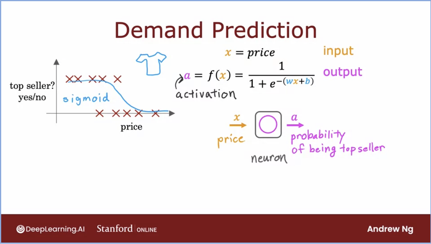
- Lets look at the image below, we have our graph with the data and it’s represented by a sigmoid function since we’ve applied logistic regression.
- Our function, which we originally called the output of the learning algorithm, we will now denote with \(a\) and call this the activation function.
- What the activation function does is it takes in the \(x\) which in our case is the price, runs the formula we see, and returns the probability that this shirt is a top seller.
- Now lets talk about how our neural network will work before we get to the activation function/output.
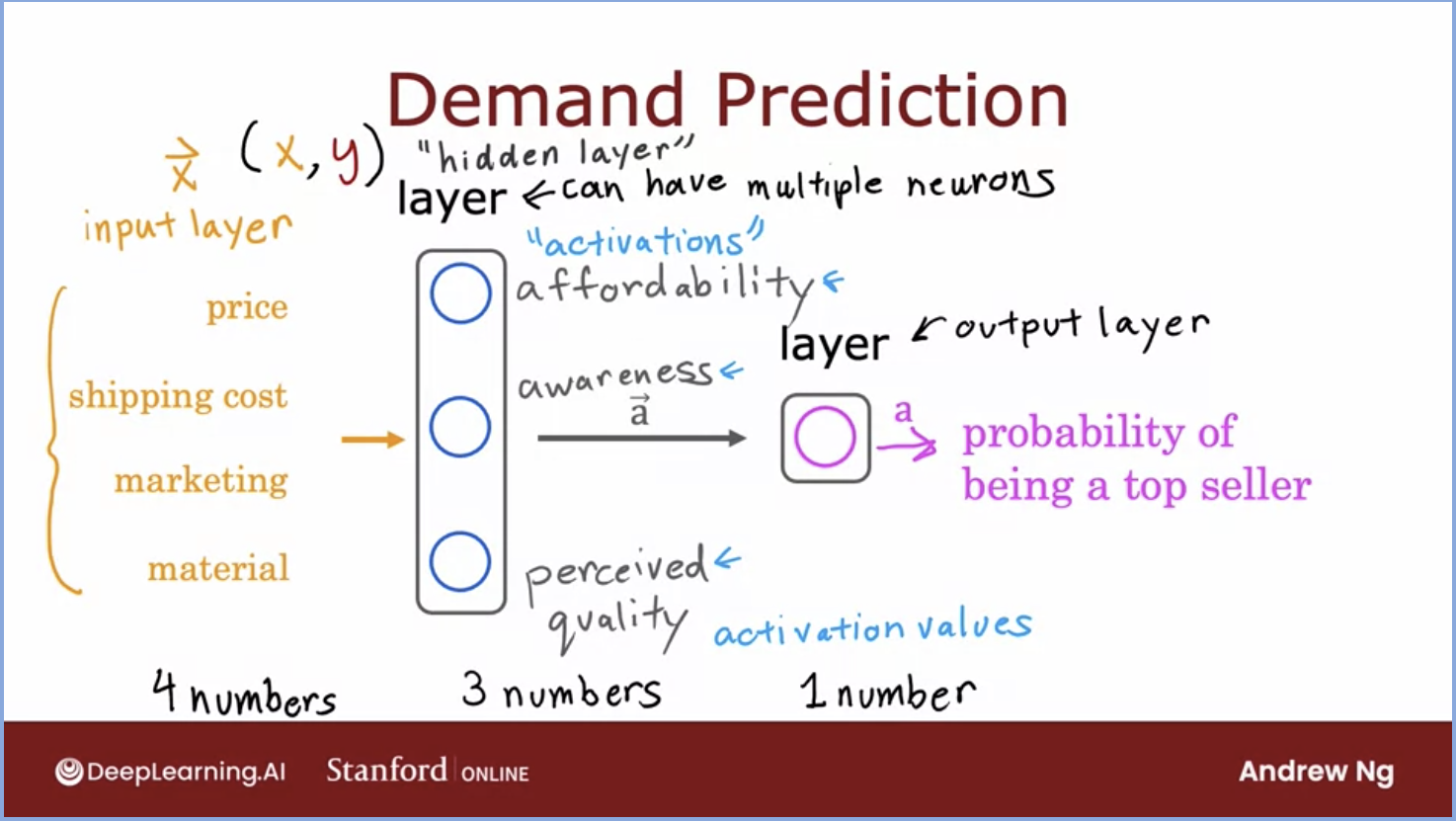
- The network will take in several features (price, marketing, material, shipping cost) \(\rightarrow\) feed it through a layer of neurons which will output \(\rightarrow\) affordability, awareness, perceived value which will output \(\rightarrow\) the probability of being the top seller.
- Each of these tasks contains a combination of neurons or a single neuron called a “layer”.
- The last layer is called the output layer, easy enough! The first layer is called the input layer that takes in a feature vector \(x\). The layer in the middle is called the hidden layer because the values for affordability,awareness etc. are not explicitly stated in the dataset.
- Each layer of neurons will have access to its previous layer and will focus on the subset of features that are the most relevant.
Neural network layer
- The fundamental building block of modern neural networks is a layer of neurons.
- How does a neural network work?
- Every layer inputs a vector of numbers and applies a bunch of logistic regression units to it, and then computes another vector of numbers. These vectors then get passed from layer to layer until you get to the final output layers computation, which is the prediction of the neural network. Then you can either threshold at 0.5 or not to come up with the final prediction.
- The conventional way to count the layers in a neural network is to count all the hidden layers and the output layer. We do not include the input layer here.
Forward Propogation
- Inference: inference is the process of using a trained model to make predictions against previously unseen data set.
- Forward propogation: going through each layer from left to right
- With forward prop, you’d be able to download the parameters of a neural network that someone else had trained and posted on the Internet. You’d also be able to carry out inference on your new data using their neural network.
- Lets look at an example with TensorFlow below:
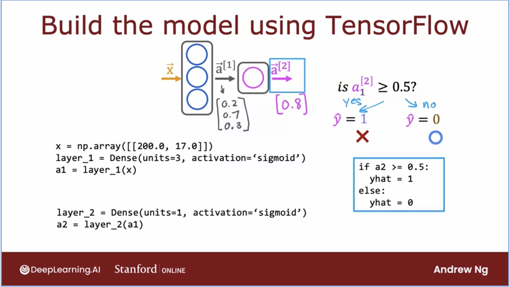
- In this image above, we can see \(x\) the input vector is instantiated as a NumPy array.
- layer_1, which is the first hidden layer in this network, is named Dense and its activation function is the \(\sigma\) function as this is a logistic regression problem.
- layer_1 can also be thought of as a function and \(a1\) will take that function with the input feature vector and hold the output vectors from that layer.
- This process will continue for the second layer and onwards.
- Each layer is carrying out inference for the layer before it.
Building a Neural Network in TensorFlow
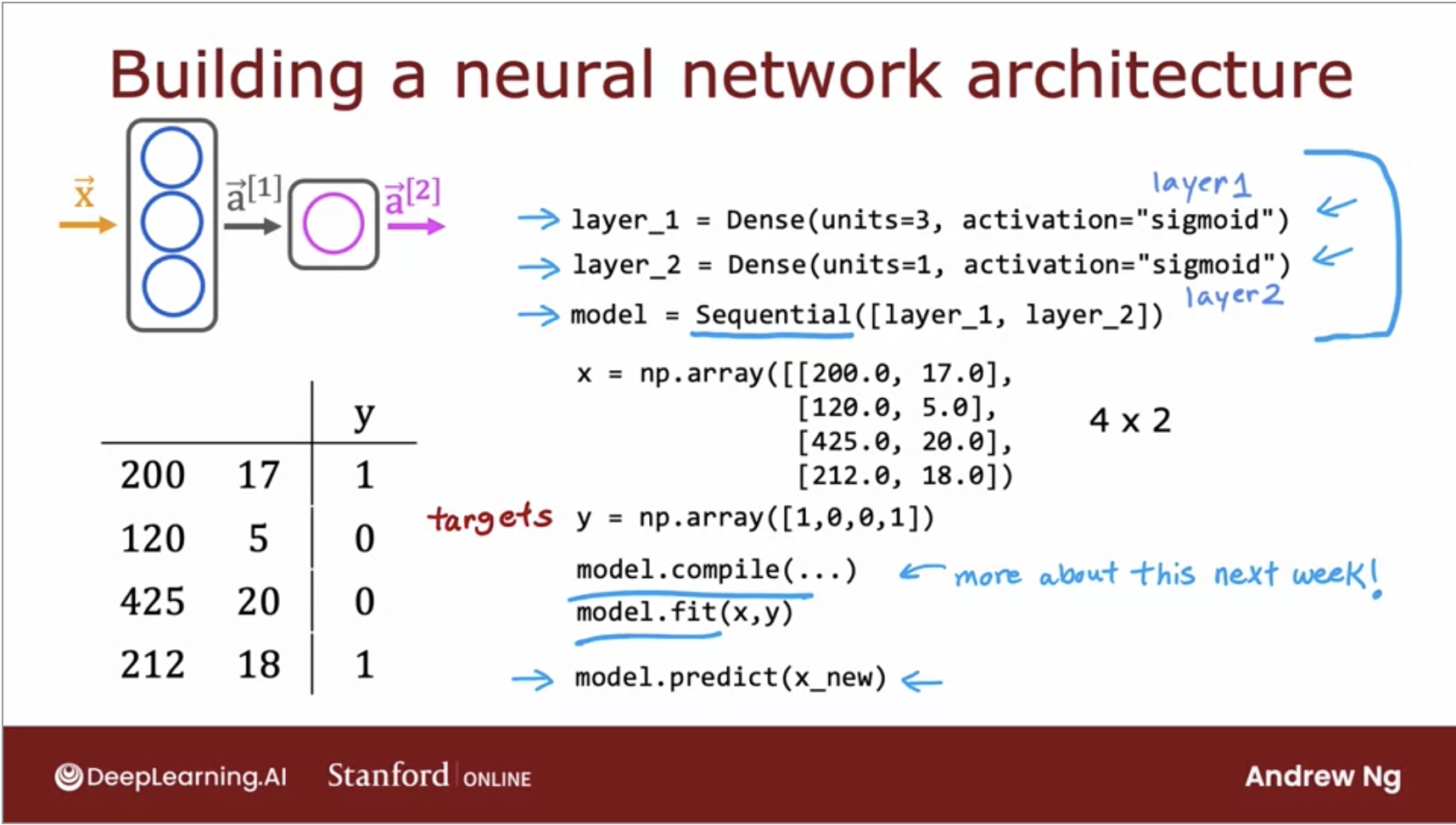
- If you want to train this neural network, all you need to do is call two functions:
model.compile() with some parameters and model.fit(x,y) which tells TensorFlow to take this neural network that are created by sequentially string together layers one and two, and to train it on the data, \(x\) and \(y\).
- Another improvement from our earlier code, instead of doing each layer sequentially, we can call \(model.predict(x_new)\) and it will output the value for \(a2\) for you given the \(new x\).
- Below is the way we would represent this in code:
- And below is a more succint version of the code doing the same thing as earlier.
Implement Forward Prop from scratch
- We’ve seen how to leverage TensorFlow, but let’s look under the hood how these would work. This will help in the future, debugging errors in your future projects.
- At a very high level, for each layer, you would need to create arrays for the parameters \(w,b\) per layer.
- Each of these would be a NumPy array and we would then have to take their dot product into our value of \(z\).
- This value \(z\) will then be given to the sigmoid function and the result would be the output vector for that layer.
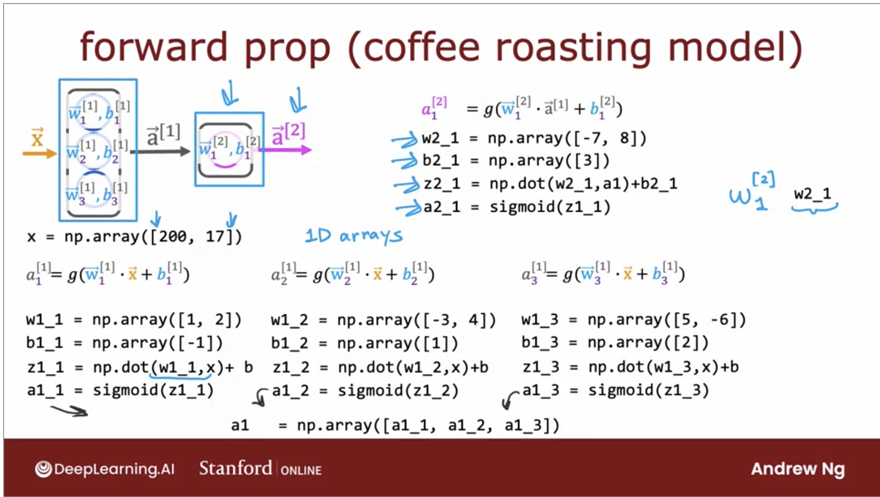
- Let’s delve even deeper, lets see how things work under the hood withing NumPy.
- Here we would need to take each neuron and create a matrix for \(w\) and \(b\).
- We would then also need to implement the dense function in python that takes in \(a, W, b, g\).
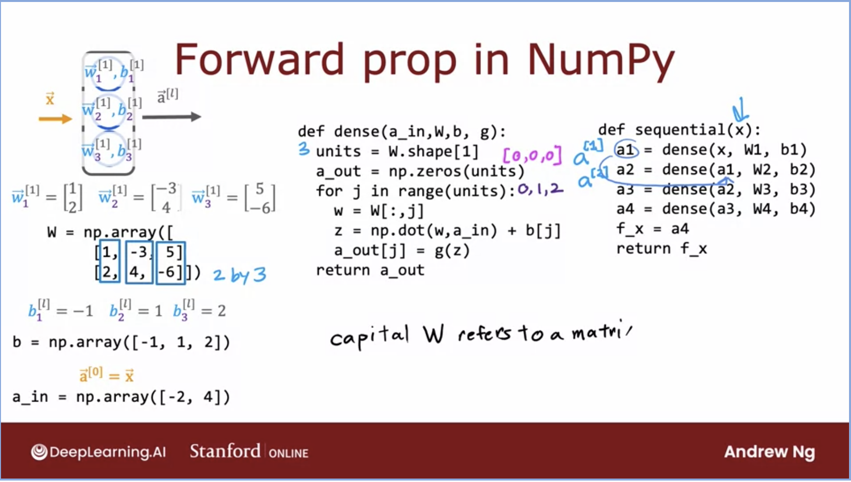
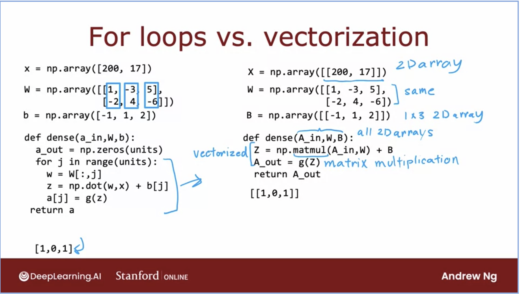
- Below is code for a vectorized implementation of forward prop in a neural network.
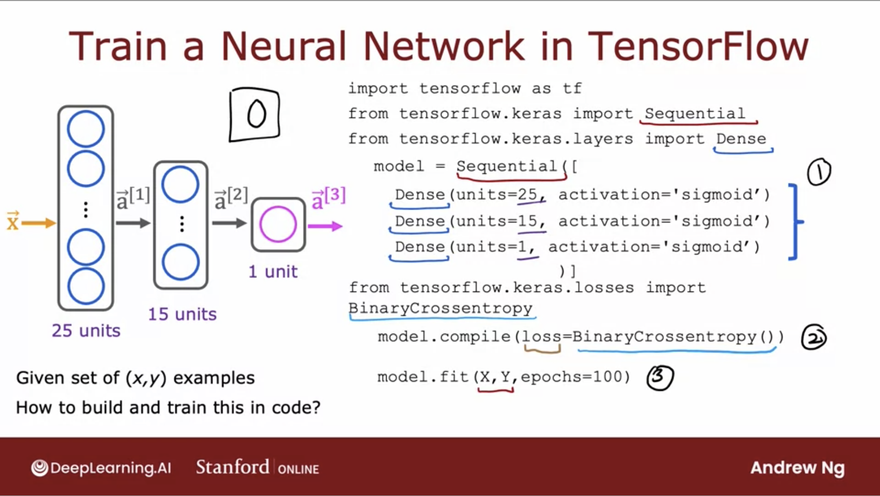
Train a Neural Network in TensorFlow
- Just an aside, a basic neural network is also called a multilayer perceptron.
- We will have the same code that we have seen before, except now we will also add the loss function.
- Here, we use
model.compile() and give it BinaryCrossentropy() as its loss value.
- After that, we will call
model.fit() which tells TensorFlow to fit the model that you specified in step 1 using the loss of the cost function that you specified in step 2 to the dataset x, y.
- Note, that epochs here tells us the number of steps to run our model, like the number of steps to run gradient descent for.
- Lets look in greater detail of how to train a neural network. First, a quick review of what we’ve seen so far:
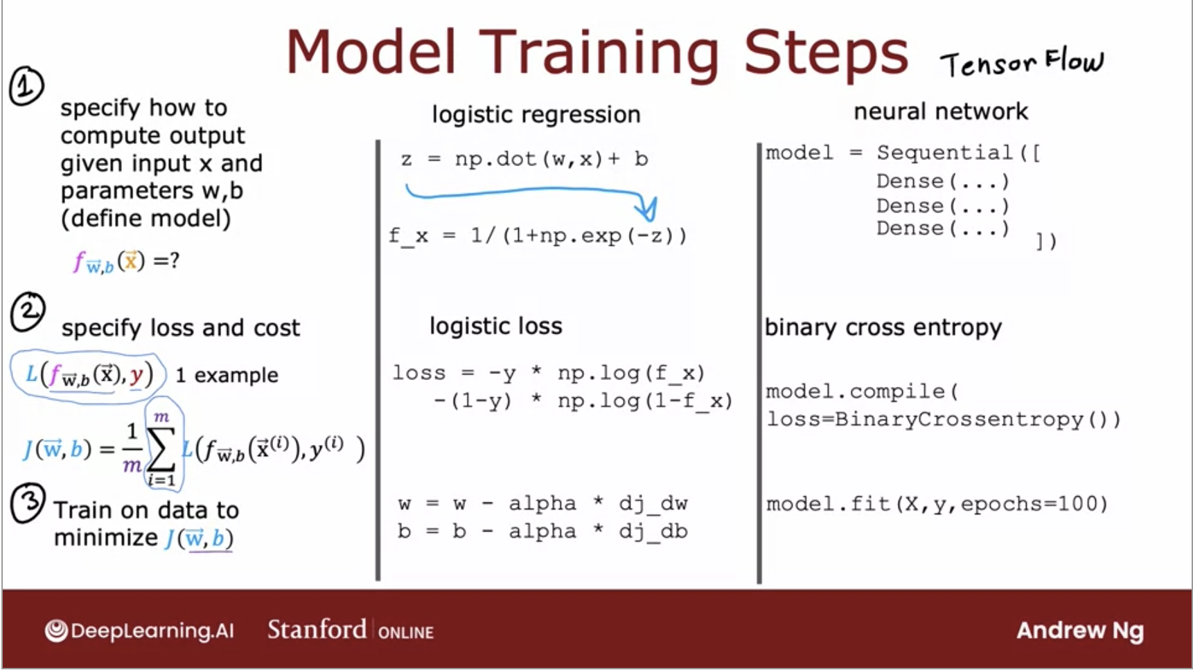
- Now lets look into each of these steps for a neural network.
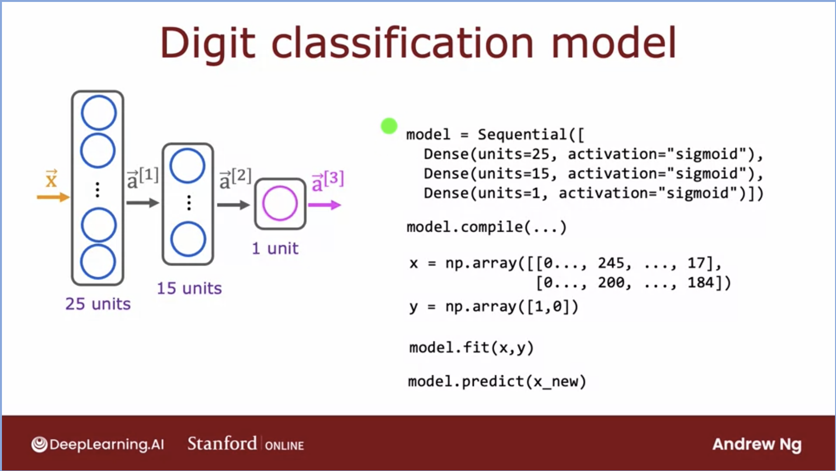
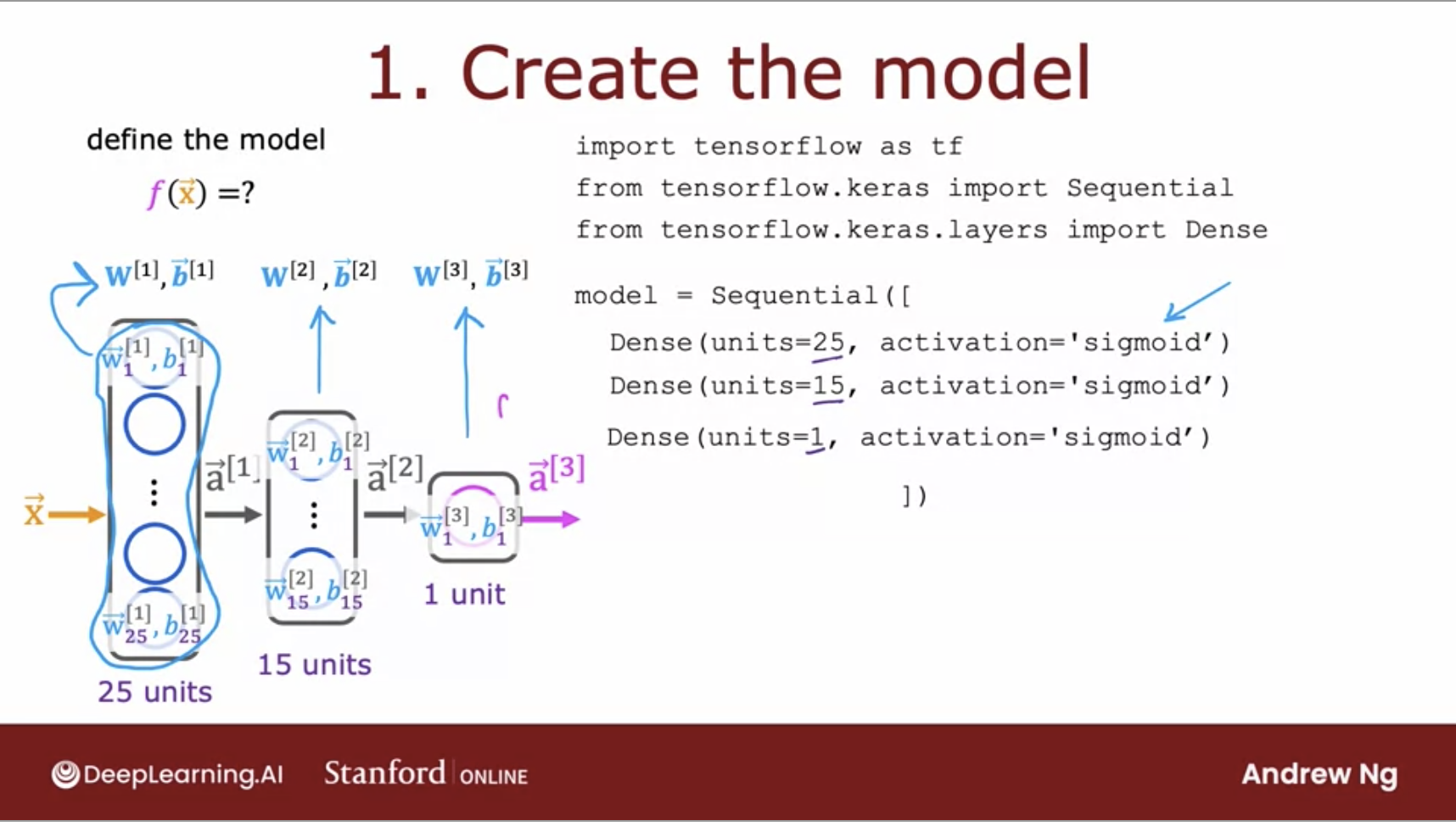
- The first step is to specify how to compute the output given the input \(x\) and parameters \(w\) and \(b\).
- This code snippet specifies the entire architecture of the neural network. It tells you that there are 25 hidden units in the first hidden layer, then the 15 in the next one, and then one output unit and that we’re using the sigmoid activation value.
- Based on this code snippet, we know also what are the parameters \(w1\), \(v1\) though the first layer parameters of the second layer and parameters of the third layer.
- This code snippet specifies the entire architecture of the neural network and therefore tells TensorFlow everything it needs in order to compute the output \(x\) as a function.
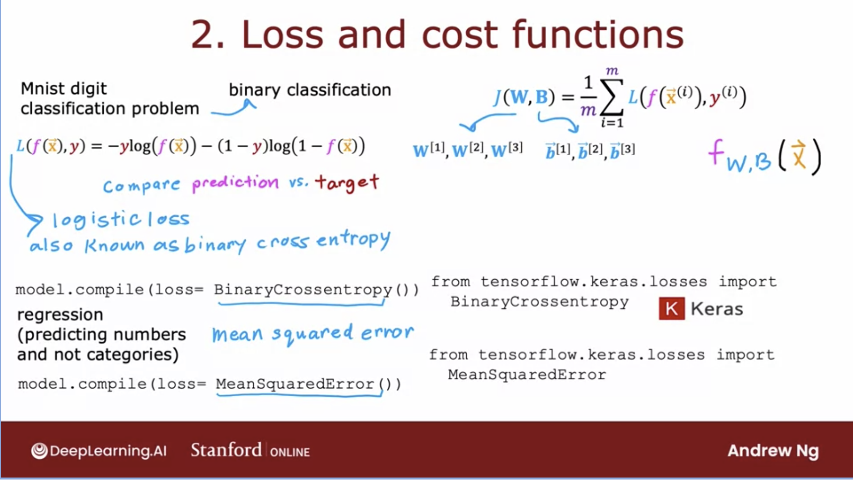
- The second step is to specify the loss/cost function we used to train the neural network.
- Btw, once you’ve specified the loss with respect to a single training example, TensorFlow will know that the cost you want to minimize is the average.
- It will take the average over all the training examples.
- You can also always change your loss function.
- The last step is to ask TensorFlow to minimize the cost function
- Remember gradient descent from earlier.
- TensorFlow will compute derivatives for gradient descent using backpropogation.
- It will do all of this using
model.fit(X,y,epochs=100).
Activation Functions
- ReLU (Rectified Linear Unit)
- Most common choice, its faster to compute and Prof. Andrew Ng suggests using it as a default for all hidden layers.
- It only goes flat in one place, thus gradient descent is faster to run.
- If the output can never be negative, like the price of a house, this is the best activation function.
- There are variants like LeakyReLU.
- Linear activation function:
- Output can be negative or positive.
- This is great for regression problems
- Sometimes if we use this, people will say we are not using any activation function.
- Sigmoid activation function:
- This is the natural choice for a binary classification problem as it will naturally give you a 0 or 1.
- It’s flat in two places so its slower than ReLU.
Multiclass Classification problem
- This is a problem where there are more than 2 classes. This is when the target \(y\) can take on more than two possible values for its output.
- Binary classification only has 2 class possibilities, whereas multiclass can have multiple possibilities for the output.
- So now we need a new decision boundary algorithm to learn the probabilities for each class.
Softmax regression algorithm
- The softmax regression algorithm is a generalization of logistic regression, which is a binary classification algorithm to the multiclass classification contexts.
- Basically, softmax is to multiclass what logistic regression is to binary classes.
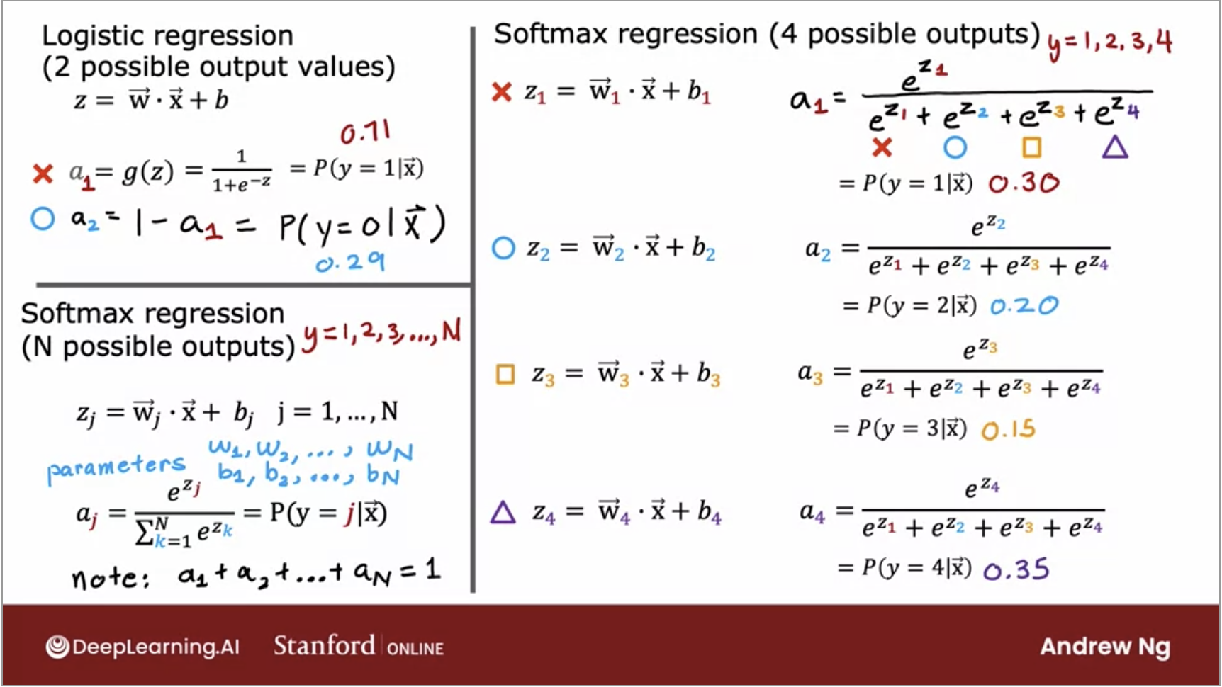
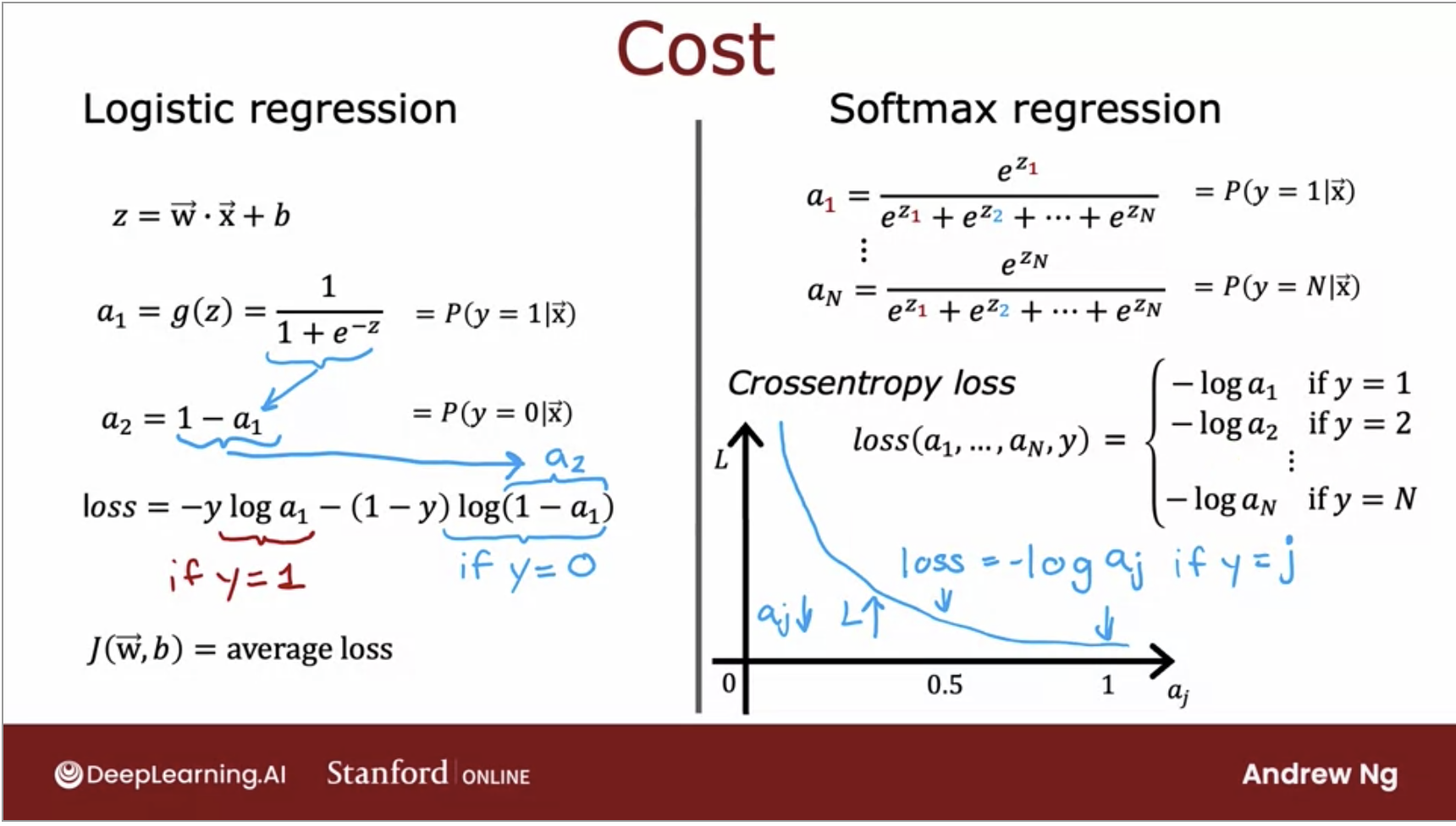
- And below is the cost function side by side for both logistic regression and softmax regression.
- In order to build a neural network to have multiclass classification, we will need to add a softmax layer to its output.
- Lets also look at the TensorFlow code for softmax below:
Convolutional Neural Network
- Recap: the dense layer we’ve been using, the activation of a neuron is a function of every single activation value from the previous layer.
- However, there is another layer type: a convolutional layer.
- Convolutional Layer only looks at part of the previous layers inputs instead of all of them. Why? We would have faster compute time and need less training data so thus would be less prone to overfitting.
- Yan LeCum was the researcher who figured out a lot of the details of how to get convolutional layers to work and popularized their use.
- Convolutional Neural Network: multiple convolutional layers in a network.
Decision Tree Learning
- You can think of a decision tree like a flow chart, it can help you make a decision based on previous experience.
- From each node, you will have two possible outcomes and it will rank the possibility of each outcome for you.
- When building a decision tree, the way we’ll decide what feature to split on at a node will be based on what choice of feature reduces entropy the most. Reduces entropy or reduces impurity, or maximizes purity.
- Information gain = reduction of entropy. Information gain lets you decide how to choose one feature to split a one-node.
- Tree ensemble: multiple decision trees collection. Sampling with replacement is how we build tree ensembles.
- Decision trees work well on tabular or structured data, something that can be stored well in an excel sheet.
- Does not work well on images, audio, text, Neural nets work better here.
- Interpretability is high, especially if the tree is small.
Random Forest Algorithm:
- A random forest is a technique that’s used to solve regression and classification problems.
- It utilizes ensemble learning, which is a technique that combines many classifiers to provide solutions to complex problems.
- It has many decision trees, the “forest” is generated by the random forest algorithm.
XGBoost
- Extreme Gradient Boosting or XGBoost is a distributed gradient-boosted decision tree.
- It provides parallel tree boosting and is the leading machine learning library for regression, classification, and ranking problems.
- It has built in regularization to prevent overfitting.
from xgboost import XGBClassifier or from XGBoost import XGBRegressor for classification vs. regression.
TL;DR
- Lets quickly go over the key takeaways from this section:
- Neural Nets behind the hood:
- Every layer inputs a vector of numbers and applies a bunch of logistic regression units to it, and then computes another vector of numbers.
- These vectors then get passed from layer to layer until you get to the final output layers computation, which is the prediction of the neural network.
- Then you can either threshold at 0.5 or not to come up with the final prediction.
- Convolutional Layer only looks at part of the previous layers inputs instead of all of them.
- They have faster compute time and need less training data so thus, are less prone to overfitting.