Distilled • LeetCode • Topological Sort
- Pattern: Topological Sort
Pattern: Topological Sort
- Overview:
- Often, in life and work, the order in which we do things is important. Every task requires completing a few prerequisite tasks first. For example, to eat food, we need to buy groceries, prep the ingredients, cook the food, clean the plates, and finally serve the food on the plates before we can eat it. We can’t prep the ingredients before we buy them. But we can clean the plates first or buy groceries first as they have no tasks that must be done before they can be attempted.
- This is the essence of the topological sort. We have a list of tasks, where some tasks have a condition that some other tasks must occur before them. Such tasks can be visualized as a graph with directed edges.
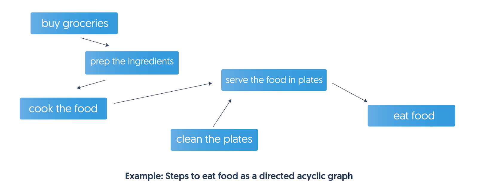
- Here, the nodes in the directed graph represent the tasks, and the directed edges between nodes tell us which task has to be done before the other. With the tasks and dependencies represented as a directed graph, we can use topological sort and find all the possible valid ways to complete a task.
- Similarly, when we are scheduling jobs or tasks, they may have dependencies. For example, before we finish task
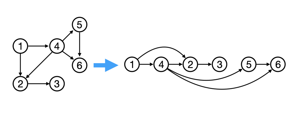
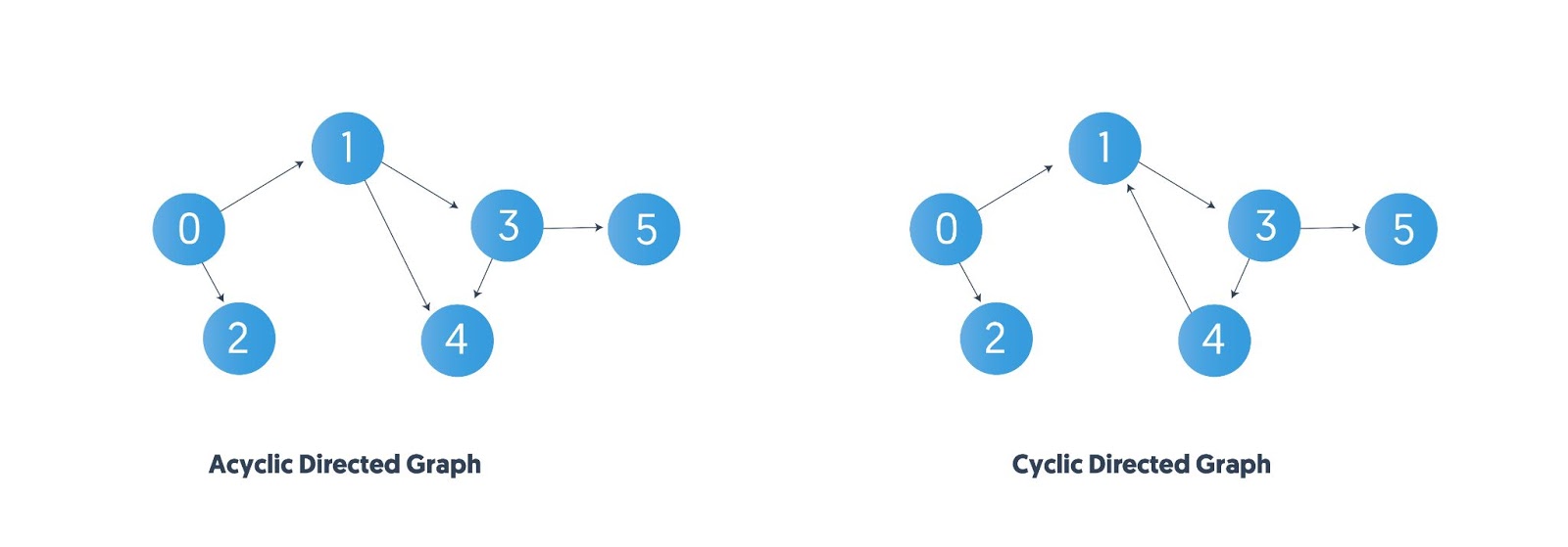
a, we have to finishbfirst. In this case, given a set of tasks and their dependencies, how shall we arrange our schedules? There comes an interesting graph algorithm: Topological Sort. - According to Introduction to Algorithms, given a directed acyclic graph (DAG), for every directed edge
(u, v), vertexucomes before vertexvin the topologically sorted order. Another way to describe it is that when you put all vertices horizontally on a line, all of the edges are pointing from left to right. Topological sorting is thus a linear ordering defined for vertices of a directed acyclic graph (DAG). This means that topological sorting for a cyclic graph is not possible. Also, there may be multiple valid topological orderings possible for the same DAG as mentioned above.
- Note that topological sort, or top sort, is defined only for directed acyclic graphs (DAGs).
- Applications of Topological Sort:
- Topological sorting is used mainly when tasks or items have to be ordered, where some tasks or items have to occur before others can. For example:
- Scheduling jobs
- Course arrangement in educational institutions
- Compile-time build dependencies
- Topological sorting is used mainly when tasks or items have to be ordered, where some tasks or items have to occur before others can. For example:
- Implementations:
- There are two ways to implement it: Breadth-First-Search (BFS) and Depth-First-Search (DFS).
- Even though Topological Sort can be implemented using both BFS and DFS, BFS is the preferred method. In some problems, the DFS route appears to be a “huge detour” and makes solutions inordinately complicated.
- BFS
- For BFS, we need an array
indegreeto keep the track of indegrees. Then we will try to output all nodes with 0 indegree, and remove the edges coming out of them at the same time. Besides, remember to put the nodes that become 0 indegree in the queue. - Then, we can keep doing this until all nodes are visited. To implement it, we can store the graph in an adjacent list (a hashmap or a dictionary in Python) and a queue to loop. - Pseudocode is demonstrated here: ``` indegree = an array indicating indegrees for each node neighbours = a HashMap recording neighbours of each node queue = [] for i in indegree: if indegree[i] == 0: queue.append(i)
while !queue.empty(): node = queue.dequeue() for neighbour in neighbours[node]: indegree[neighbour] -= 1 if indegree[neighbour] == 0: queue.append(neighbour) ```
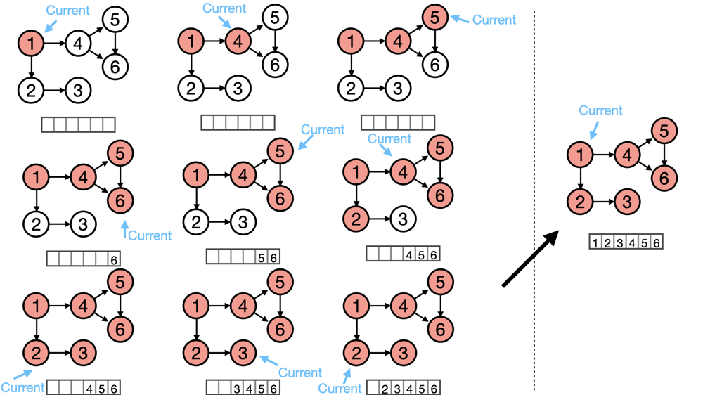
- The following figure illustrates topological Sort with BFS:
- For BFS, we need an array
- DFS
- The key observation is that, leaf nodes should always come after their parents and ancestors. Following this intuition we can apply DFS and output nodes from leaves to the root.
- We need to implement a boolean array visited so that
visited[i]indicates if we have visited vertexi. For each unvisited node, we would first mark it as visited and callDFS()to start searching its neighbors. After finishing this, we can insert it to the front of a list. After visiting all nodes, we can return that list.
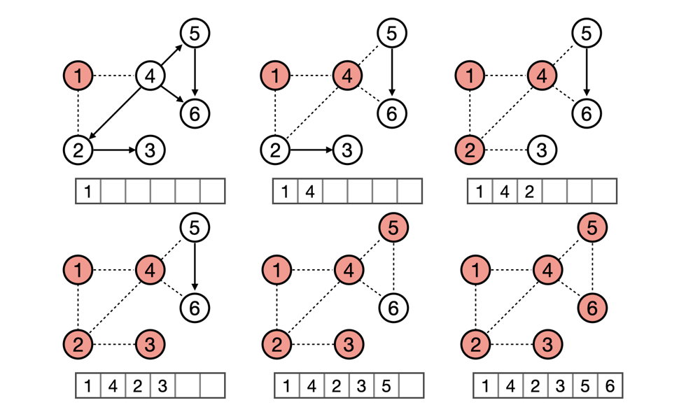
def topological_sort(): for each node: if visited[node] is False: dfs(node) def dfs(node): visited[node] = True for nei in neighbours[node]: dfs(nei) if visited(node) = false: ret.insert_at_the _front(node)- The following figure illustrates topological Sort with DFS:
- BFS
- Kahn’s Algorithm for Topological Sorting:
- Kahn’s algorithm takes a directed acyclic graph and sorts its nodes in topological order. It works by keeping track of the number of incoming edges into each node, also called in-degree. It repeatedly:
- Finds nodes with no incoming edge, that is, nodes with zero in-degree (no dependency)
- Stores the nodes with zero in-degree
- Removes all outgoing edges from the nodes with zero in-degree
- Decrements the in-degree for each node after a connected edge removal
- (Steps 3 and 4 can be performed simultaneously.)
- This process is done until no element with zero in-degree can be found. This can happen when the topological sorting is complete and also when a cycle is encountered. Therefore, the algorithm checks if the result of topological sorting contains the same number of elements that were supposed to be sorted:
- If the numbers match, then no cycle was encountered, and we print the sorted order.
- If a cycle was encountered, the topological sorting was not possible. This is conveyed by returning null or printing a message.
- Example:

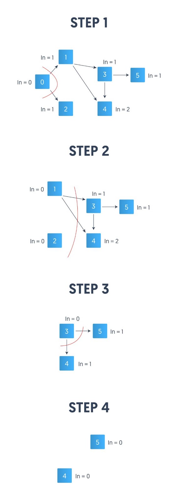
- Here, “In” = indegree
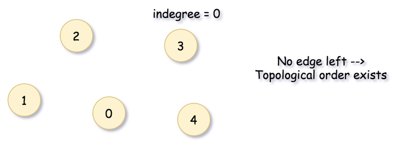
- Order of removal: First 0, then 1 and 2, then 3, and finally, 4 and 5.
- Topological order: 0,1,2,3,4,5
- Note: This is not the only possible topological order. For example, 0,1,3,4,5,2 is also a valid topological order.
- Kahn’s algorithm takes a directed acyclic graph and sorts its nodes in topological order. It works by keeping track of the number of incoming edges into each node, also called in-degree. It repeatedly:
- Why Topological Sort Does Not Work for Cyclic Graphs:
- If we had no clothes to go out, and we needed to go out to get clothes, we would be in a cycle where one task depends on the other, and no task independent of a prerequisite exists. Therefore, we can’t begin!
- This is why topological sorting doesn’t work for cyclic graphs. In any graph where there’s a cycle, there comes a time where there’s no node left that is devoid of dependencies.
- Topological Sort Example Using Kahn’s Algorithm:
- To understand the process more concretely, let’s take an example:
Edges: { 0, 1 }, { 0, 2 }, { 1, 3}, {1, 4), { 3, 4}, { 3, 5 }
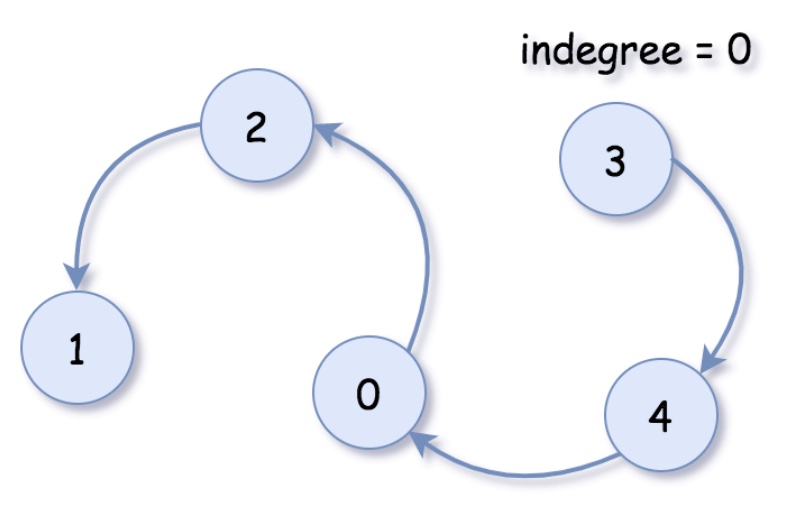
- We now calculate the indegree of each node. The indegree of a node pictorially refers to the number of edges pointing towards that node. The direction of the arrow is incoming, hence the term indegree.
-
In terms of edges, each edge \({U_i, V}\) where \(U_i\) is the source and \(V\) is the destination node contributes to the indegree of its destination node V as the edge points towards it. We’re going to update the indegree value for any node \(V\) every time an edge associated with it as its destination node is deleted.
- Node 0 has zero incoming edges. In = 0
- Nodes 1,2,3, and 5 have one incoming edge. In = 1
- Node 4 has two incoming edges. In = 2
- We can now begin applying Kahn’s algorithm for topological sorting.
- Overall the process is as follows:
- In this example, we start with the node with in-degree zero, remove that node and its edges, add it to our sorted list.
- Then, we decrement the in-degrees of the nodes it was connected to and repeat all these steps until all elements are sorted. Note that there may exist more than one valid topological ordering in an acyclic graph, as is the case in this example as well.
- Step-by-step process:
- Step 1: The indegree of node 0 is zero. This is the only node with indegree zero at the beginning. We remove this node and its outward edges: {0, 1}, {0, 2}
- Step 2: We update the indegree of the deleted edges’ destination nodes. Directed edges contribute to the indegree of their destination nodes, as they are pointing towards them. Now the indegree of nodes 1 and 2 both are decremented by one. Since the indegree before this decrement for both nodes was 1, this also makes node 1 and node 2 the new nodes with indegree zero. We now remove these two nodes. Node 2 has no outgoing edges. Node 1 has two outgoing edges, so we also remove those: {1, 3}, {1, 4}
- Step 3: We now decrement the indegrees of destination nodes of these edges 3 and 4. Hence the indegree of node 4 goes from 2 to 1, and the indegree of node 3 goes from 1 to 0. This makes node 3 the new node to remove. We also remove its outgoing edges: {3, 4},{3, 5}
- Step 4: We update the indegrees of the destination nodes of the deleted edges. So the indegrees of node 4 and node 5, which were both 1 before the decrement, now become zero. We are now left with only these two nodes: node 4 and node 5, both with indegree zero and no outgoing edges from either node. When multiple nodes have indegree zero at the same time, we can write either one before the other.
- Step 5: There may be multiple topological orderings possible in an acyclic graph, as is the case in this example as well. We repeat this process till all nodes are sorted and output one of these valid topological orderings. A valid topological ordering we end up with here is 0,1,2,3,4,5.
- Overall the process is as follows:
- To understand the process more concretely, let’s take an example:
- Topological Sort Algorithm:
- Now that we’ve looked at Kahn’s Algorithm for topological sorting in detail with an example, we can condense it as the topological sort algorithm:
- Step 0: Find indegree for all nodes.
- Step 1: Identify a node with no incoming edges.
- Step 2: Remove the node from the graph and add it to the ordering.
- Step 3: Remove the node’s out-going edges from the graph.
- Step 4: Decrement the in-degree where connected edges were deleted.
- Step 5: Repeat Steps 1 to 4 till there are no nodes left with zero in-degree.
- Step 6: Check if all elements are present in the sorted order.
- Step 7: If the result of Step 6 is true, we have the sorted order. Else no topological ordering exists.
- Step 8: Exit.
- Now that we’ve looked at Kahn’s Algorithm for topological sorting in detail with an example, we can condense it as the topological sort algorithm:
- Typical Complexity for Topological Sort:
- Time: \(O(\midV\mid+\midE\mid)\)
- Space: \(O(\midV\mid+\midE\mid)\)
[207/Medium] Course Schedule
Problem
- There are a total of numCourses courses you have to take, labeled from
0tonumCourses - 1. You are given an array prerequisites whereprerequisites[i] = [ai, bi]indicates that you must take coursebifirst if you want to take courseai.- For example, the pair
[0, 1], indicates that to take course 0 you have to first take course 1.
- For example, the pair
-
Return
trueif you can finish all courses. Otherwise, returnfalse. - Example 1:
Input: numCourses = 2, prerequisites = [[1,0]]
Output: true
Explanation: There are a total of 2 courses to take.
To take course 1 you should have finished course 0. So it is possible.
- Example 2:
Input: numCourses = 2, prerequisites = [[1,0],[0,1]]
Output: false
Explanation: There are a total of 2 courses to take.
To take course 1 you should have finished course 0, and to take course 0 you should also have finished course 1. So it is impossible.
- Constraints:
1 <= numCourses <= 20000 <= prerequisites.length <= 5000prerequisites[i].length == 20 <= ai, bi < numCoursesAll the pairs prerequisites[i] are unique.
- See problem on LeetCode.
Solution: Backtracking
- Intuition:
- The problem could be modeled as yet another graph traversal problem, where each course can be represented as a vertex in a graph and the dependency between the courses can be modeled as a directed edge between two vertex.
And the problem to determine if one could build a valid schedule of courses that satisfies all the dependencies (i.e. constraints) would be equivalent to determine if the corresponding graph is a DAG (Directed Acyclic Graph), i.e. there is no cycle existed in the graph.

-
A typical strategy for graph traversal problems would be backtracking or simply DFS (depth-first search).
-
Here let us start with the backtracking algorithm, which arguably might be more intuitive.
As a reminder, backtracking is a general algorithm that is often applied to solve the constraint satisfaction problems, which incrementally builds candidates to the solutions, and abandons a candidate (i.e. backtracks) as soon as it determines that the candidate would not lead to a valid solution.
-
The general idea here is that we could enumerate each course (vertex), to check if it could form cyclic dependencies (i.e. a cyclic path) starting from this course.
-
The check of cyclic dependencies for each course could be done via backtracking, where we incrementally follow the dependencies until either there is no more dependency or we come across a previously visited course along the path.
- Algorithm:
- The overall structure of the algorithm is simple, which consists of three main steps:
- We build a graph data structure from the given list of course dependencies. Here we adopt the adjacency list data structure as shown below to represent the graph, which can be implemented via hashmap or dictionary. Each entry in the adjacency list represents a node which consists of a node index and a list of neighbors nodes that follow from the node.

- We then enumerate each node (course) in the constructed graph, to check if we could form a dependency cycle starting from the node.
- We perform the cyclic check via backtracking, where we breadcrumb our path (i.e. mark the nodes we visited) to detect if we come across a previously visited node (hence a cycle detected). We also remove the breadcrumbs for each iteration.
- We build a graph data structure from the given list of course dependencies. Here we adopt the adjacency list data structure as shown below to represent the graph, which can be implemented via hashmap or dictionary. Each entry in the adjacency list represents a node which consists of a node index and a list of neighbors nodes that follow from the node.
- The overall structure of the algorithm is simple, which consists of three main steps:
- Implementation:
class Solution(object):
    def canFinish(self, numCourses, prerequisites):
        """
        :type numCourses: int
        :type prerequisites: List[List[int]]
        :rtype: bool
        """
        from collections import defaultdict
        courseDict = defaultdict(list)

        for relation in prerequisites:
            nextCourse, prevCourse = relation[0], relation[1]
            courseDict[prevCourse].append(nextCourse)

        path = [False] * numCourses
        for currCourse in range(numCourses):
            if self.isCyclic(currCourse, courseDict, path):
                return False
        return True

    def isCyclic(self, currCourse, courseDict, path):
        """
        backtracking method to check that no cycle would be formed starting from currCourse
        """
        if path[currCourse]:
            # come across a previously visited node, i.e. detect the cycle
            return True

        # before backtracking, mark the node in the path
        path[currCourse] = True

        # backtracking
        ret = False
        for child in courseDict[currCourse]:
            ret = self.isCyclic(child, courseDict, path)
            if ret: break

        # after backtracking, remove the node from the path
        path[currCourse] = False
        return ret
Complexity
-
Time: $$\mathcal{O}( E + V ^ 2)\(where\) E \(is the number of dependencies,\) V $$ is the number of courses and dd is the maximum length of acyclic paths in the graph. -
First of all, it would take us $$ E $$ steps to build a graph in the first step. - For a single round of backtracking, in the worst case where all the nodes chained up in a line, it would take us maximum \(|V|\) steps to terminate the backtracking.

-
Again, follow the above worst scenario where all nodes are chained up in a line, it would take us in total $$\sum_{i=1}^{ V }{i} = \frac{(1+ V )\cdot V }{2}$$ steps to finish the check for all nodes. -
As a result, the overall time complexity of the algorithm would be $$\mathcal{O}( E + V ^ 2)$$.
-
-
Space: $$\mathcal{O}( E + V )$$, with the same denotation as in the above time complexity. -
We built a graph data structure in the algorithm, which would consume $$ E + V $$ space. -
In addition, during the backtracking process, we employed a sort of bitmap (path) to keep track of all visited nodes, which consumes $$ V $$ space. -
Finally, since we implement the function in recursion, which would incur additional memory consumption on call stack. In the worst case where all nodes are chained up in a line, the recursion would pile up $$ V $$ times. -
Hence the overall space complexity of the algorithm would be $$\mathcal{O}( E + 3\cdot V ) = \mathcal{O}( E + V )$$.
-
Solution: Postorder DFS (Depth-First Search)
- Intuition:
- As one might notice that, with the above backtracking algorithm, we would visit certain nodes multiple times, which is not the most efficient way.
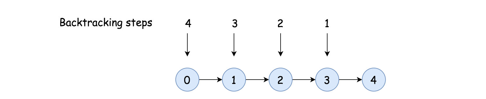
- For instance, in the above graph where the nodes are chained up in a line, the backtracking algorithm would end up of being a nested two-level iteration over the nodes, which we could rewrite as the following pseudo code:
for i in range(0, len(nodes)): # start from the current node to check if a cycle might be formed. for j in range(i, len(nodes)): isCyclic(nodes[j], courseDict, path) - One might wonder that if there is a better algorithm that visits each node once and only once. And the answer is yes.
- In the above example, for the first node in the chain, once we’ve done the check that there would be no cycle formed starting from this node, we don’t have to do the same check for all the nodes in the downstream.
The rationale is that given a node, if the subgraph formed by all descendant nodes from this node has no cycle, then adding this node to the subgraph would not form a cycle either.
- From the perspective of graph traversal, the above rationale could be implemented with the strategy of postorder DFS (depth-first search), in which strategy we visit a node’s descendant nodes before the node itself.
- As one might notice that, with the above backtracking algorithm, we would visit certain nodes multiple times, which is not the most efficient way.
- Algorithm:
- We could implement the postorder DFS based on the above backtracking algorithm, by simply adding another bitmap (i.e. checked[node_index]) which indicates whether we have done the cyclic check starting from a particular node.
- Here are the breakdowns of the algorithm, where the first 2 steps are the same as in the previous backtracking algorithm.
- We build a graph data structure from the given list of course dependencies.
- We then enumerate each node (course) in the constructed graph, to check if we could form a dependency cycle starting from the node.
- We check if the current node has been checked before, otherwise we enumerate through its child nodes via backtracking, where we breadcrumb our path (i.e. mark the nodes we visited) to detect if we come across a previously visited node (hence a cycle detected). We also remove the breadcrumbs for each iteration.
- Once we visited all the child nodes (i.e. postorder), we mark the current node as checked.
- Implementation:
class Solution(object):
    def canFinish(self, numCourses, prerequisites):
        """
        :type numCourses: int
        :type prerequisites: List[List[int]]
        :rtype: bool
        """
        from collections import defaultdict
        courseDict = defaultdict(list)

        for relation in prerequisites:
            nextCourse, prevCourse = relation[0], relation[1]
            courseDict[prevCourse].append(nextCourse)

        checked = [False] * numCourses
        path = [False] * numCourses

        for currCourse in range(numCourses):
            if self.isCyclic(currCourse, courseDict, checked, path):
                return False
        return True


    def isCyclic(self, currCourse, courseDict, checked, path):
        """   """
        # 1). bottom-cases
        if checked[currCourse]:
            # this node has been checked, no cycle would be formed with this node.
            return False
        if path[currCourse]:
            # came across a marked node in the path, cyclic !
            return True

        # 2). postorder DFS on the children nodes
        # mark the node in the path
        path[currCourse] = True

        ret = False
        # postorder DFS, to visit all its children first.
        for child in courseDict[currCourse]:
            ret = self.isCyclic(child, courseDict, checked, path)
            if ret: break

        # 3). after the visits of children, we come back to process the node itself
        # remove the node from the path
        path[currCourse] = False

        # Now that we've visited the nodes in the downstream,
        #   we complete the check of this node.
        checked[currCourse] = True
        return ret
- Note, one could also use a single bitmap with 3 states such as
not_visited,visited,checked, rather than having two bitmaps as we did in the algorithm, though we argue that it might be clearer to have two separated bitmaps.
Complexity
-
Time: $$\mathcal{O}( E + V )\(where\) V \(is the number of courses, and\) E $$ is the number of dependencies. -
As in the previous algorithm, it would take us $$ E $$ time complexity to build a graph in the first step. -
Since we perform a postorder DFS traversal in the graph, we visit each vertex and each edge once and only once in the worst case, i.e. $$ E + V $$.
-
-
Space: $$\mathcal{O}( E + V )$$, with the same denotation as in the above time complexity. -
We built a graph data structure in the algorithm, which would consume $$ E + V $$ space. -
In addition, during the backtracking process, we employed two bitmaps (path and visited) to keep track of the visited path and the status of check respectively, which consumes $$2 \cdot V $$ space. -
Finally, since we implement the function in recursion, which would incur additional memory consumption on call stack. In the worst case where all nodes chained up in a line, the recursion would pile up $$ V $$ times. -
Hence the overall space complexity of the algorithm would be $$\mathcal{O}( E + 4\cdot V ) = \mathcal{O}( E + V )$$.
-
Solution: Topological Sort
- Intuition:
- Actually, the problem is also known as topological sort problem, which is to find a global order for all nodes in a DAG (Directed Acyclic Graph) with regarding to their dependencies.
- A linear algorithm was first proposed by Arthur Kahn in 1962, in his paper of “Topological order of large networks”. The algorithm returns a topological order if there is any. Here we quote the pseudo code of the Kahn’s algorithm from wikipedia as follows:
L = Empty list that will contain the sorted elements S = Set of all nodes with no incoming edge while S is non-empty do remove a node n from S add n to tail of L for each node m with an edge e from n to m do remove edge e from the graph if m has no other incoming edges then insert m into S if graph has edges then return error (graph has at least one cycle) else return L (a topologically sorted order) - To better understand the above algorithm, we summarize a few points here:
- In order to find a global order, we can start from those nodes which do not have any prerequisites (i.e., indegree of node is zero), we then incrementally add new nodes to the global order, following the dependencies (edges).
- Once we follow an edge, we then remove it from the graph.
- With the removal of edges, there would more nodes appearing without any prerequisite dependency, in addition to the initial list in the first step.
- The algorithm would terminate when we can no longer remove edges from the graph. There are two possible outcomes:
- If there are still some edges left in the graph, then these edges must have formed certain cycles, which is similar to the deadlock situation. It is due to these cyclic dependencies that we cannot remove them during the above processes.
- Otherwise, i.e. we have removed all the edges from the graph, and we got ourselves a topological order of the graph.
- Algorithm:
- Following the above intuition and pseudo code, here we list some sample implementations.
- Implementation:
class GNode(object):
    """  data structure represent a vertex in the graph."""
    def __init__(self):
        self.inDegrees = 0
        self.outNodes = []

class Solution(object):
    def canFinish(self, numCourses, prerequisites):
        """
        :type numCourses: int
        :type prerequisites: List[List[int]]
        :rtype: bool
        """
        from collections import defaultdict, deque
        # key: index of node; value: GNode
        graph = defaultdict(GNode)

        totalDeps = 0
        for relation in prerequisites:
            nextCourse, prevCourse = relation[0], relation[1]
            graph[prevCourse].outNodes.append(nextCourse)
            graph[nextCourse].inDegrees += 1
            totalDeps += 1

        # we start from courses that have no prerequisites.
        # we could use either set, stack or queue to keep track of courses with no dependence.
        nodepCourses = deque()
        for index, node in graph.items():
            if node.inDegrees == 0:
                nodepCourses.append(index)

        removedEdges = 0
        while nodepCourses:
            # pop out course without dependency
            course = nodepCourses.pop()

            # remove its outgoing edges one by one
            for nextCourse in graph[course].outNodes:
                graph[nextCourse].inDegrees -= 1
                removedEdges += 1
                # while removing edges, we might discover new courses with prerequisites removed, i.e. new courses without prerequisites.
                if graph[nextCourse].inDegrees == 0:
                    nodepCourses.append(nextCourse)

        if removedEdges == totalDeps:
            return True
        else:
            # if there are still some edges left, then there exist some cycles
            # Due to the dead-lock (dependencies), we cannot remove the cyclic edges
            return False
- Note that we could use different types of containers, such as Queue, Stack or Set, to keep track of the nodes that have no incoming dependency, i.e.
indegree = 0. Depending on the type of container, the resulting topological order would be different, though they are all valid.
Complexity
-
Time: $$\mathcal{O}( E + V )\(where\) V \(is the number of courses, and\) E $$ is the number of dependencies. -
As in the previous algorithm, it would take us $$ E $$ time complexity to build a graph in the first step. -
Similar with the above postorder DFS traversal, we would visit each vertex and each edge once and only once in the worst case, i.e. $$ E + V $$. -
As a result, the overall time complexity of the algorithm would be $$\mathcal{O}(2\cdot E + V ) = \mathcal{O}( E + V )$$.
-
-
Space: $$\mathcal{O}( E + V )$$, with the same denotation as in the above time complexity. -
We built a graph data structure in the algorithm, which would consume $$ E + V $$ space. -
In addition, we use a container to keep track of the courses that have no prerequisite, and the size of the container would be bounded by $$ V $$. -
As a result, the overall space complexity of the algorithm would be $$\mathcal{O}( E + 2\cdot V ) = \mathcal{O}( E + V )$$.
-
[210/Medium] Course Schedule II
Problem
- There are a total of numCourses courses you have to take, labeled from 0 to
numCourses - 1. You are given an array prerequisites whereprerequisites[i] = [ai, bi]indicates that you must take course bi first if you want to take courseai.- For example, the pair
[0, 1], indicates that to take course 0 you have to first take course 1.
- For example, the pair
-
Return the ordering of courses you should take to finish all courses. If there are many valid answers, return any of them. If it is impossible to finish all courses, return an empty array.
- Example 1:
Input: numCourses = 2, prerequisites = [[1,0]]
Output: [0,1]
Explanation: There are a total of 2 courses to take. To take course 1 you should have finished course 0. So the correct course order is [0,1].
- Example 2:
Input: numCourses = 4, prerequisites = [[1,0],[2,0],[3,1],[3,2]]
Output: [0,2,1,3]
Explanation: There are a total of 4 courses to take. To take course 3 you should have finished both courses 1 and 2. Both courses 1 and 2 should be taken after you finished course 0.
So one correct course order is [0,1,2,3]. Another correct ordering is [0,2,1,3].
- Example 3:
Input: numCourses = 1, prerequisites = []
Output: [0]
- Constraints:
1 <= numCourses <= 20000 <= prerequisites.length <= numCourses * (numCourses - 1)prerequisites[i].length == 20 <= ai, bi < numCoursesai != biAll the pairs [ai, bi] are distinct.
- See problem on LeetCode.
Solution: DFS
-
This is a very common problem that some of us might face during college. We might want to take up a certain set of courses that interest us. However, as we all know, most of the courses do tend to have a lot of prerequisites associated with them. Some of these would be hard requirements whereas others would be simply suggested prerequisites which you may or may not take. However, for us to be able to have an all round learning experience, we should follow the suggested set of prerequisites. How does one decide what order of courses they should follow so as not to miss out on any subjects?
-
As mentioned in the problem statement, such a problem is a natural fit for graph based algorithms and we can easily model the elements in the problem statement as a graph. First of all, let’s look at the graphical representation of the problem and it’s components and then we will move onto the solutions.
- We can represent the information provided in the question in the form of a graph.
- Let \(G(V, E)\) represent a directed, unweighted graph.
- Each course would represent a vertex in the graph.
- The edges are modeled after the prerequisite relationship between courses. So, we are given, that a pair such as
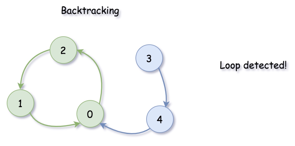
[a, b]in the question means the course b is a prerequisite for the course a. This can be represented as a directed edgeb -> ain the graph. - The graph is a cyclic graph because there is a possibility of a cycle in the graph. If the graph would be acyclic, then an ordering of subjects as required in the question would always be possible. Since it’s mentioned that such an ordering may not always be possible, that means we have a cyclic graph.
- Let’s look at a sample graph representing a set of courses where such an ordering is possible and one where such an ordering is not possible. It will be easier to explain the approaches once we look at two sample graphs.
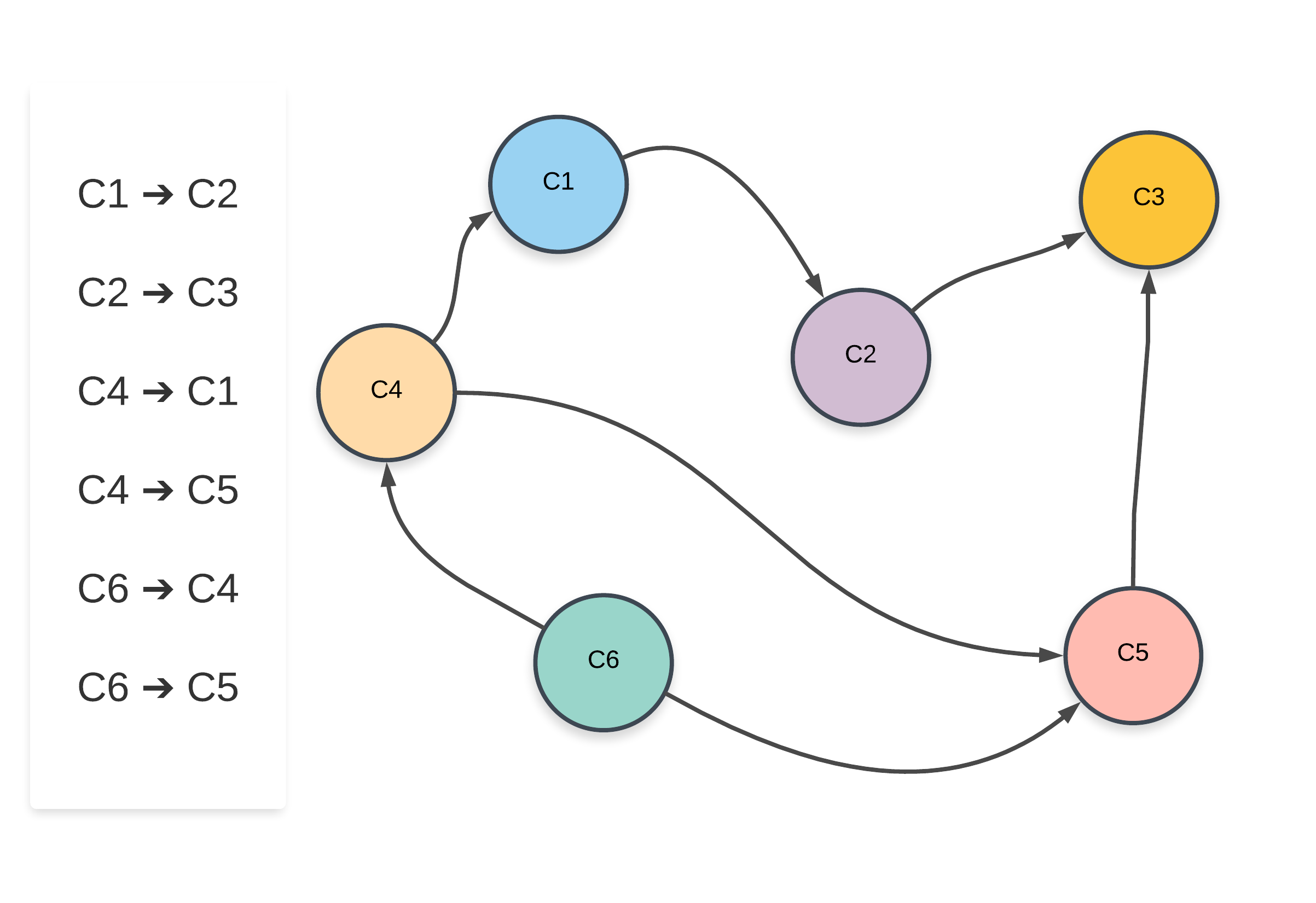
- For the sample graph shown above, one of the possible ordering of courses is:
C6 -> C4 -> C1 -> C5 -> C2 -> C3and another possible ordering of subjects isC6 -> C4 -> C5 -> C1 -> C2 -> C3. Now let’s look at a graph where no such ordering of courses is possible.
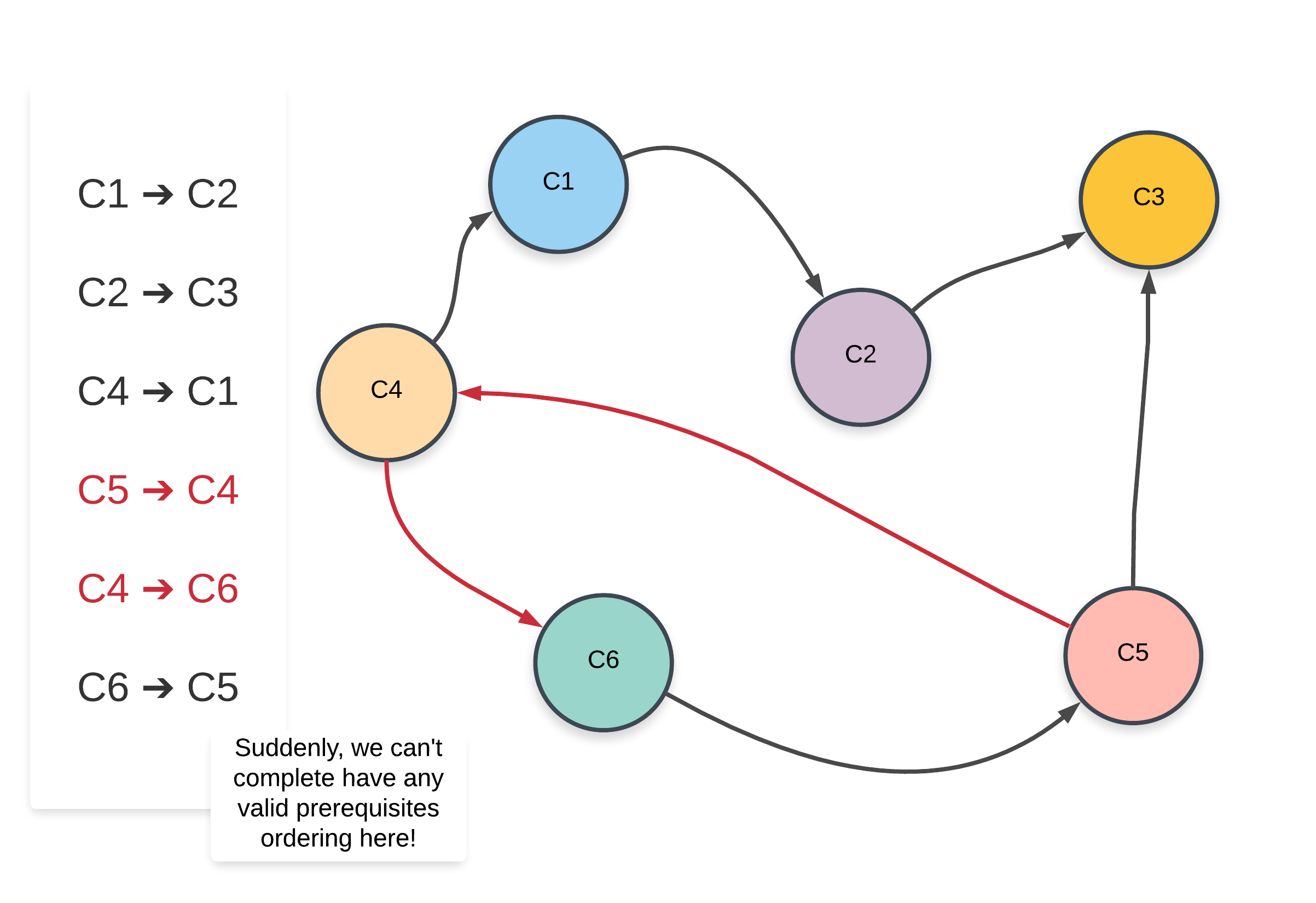
- Note that the edges that have changed from the previous graph have been highlighted in red.
Clearly, the presence of a cycle in the graph shows us that a proper ordering of prerequisites is not possible at all. Intuitively, it is not possible to have e.g. two subjects S1 and S2 prerequisites of each other. Similar ideology applies to a larger cycle in the graph like we have above.
-
Such an ordering of subjects is referred to as a Topological Sorted Order and this is a common algorithmic problem in the graph domain. There are two approaches that we will be looking at in this article to solve this problem.
- Intuition:
- Suppose we are at a node in our graph during the depth first traversal. Let’s call this node A.
The way DFS would work is that we would consider all possible paths stemming from A before finishing up the recursion for A and moving onto other nodes. All the nodes in the paths stemming from the node A would have A as an ancestor. The way this fits in our problem is, all the courses in the paths stemming from the course A would have A as a prerequisite.
- Now we know how to get all the courses that have a particular course as a prerequisite. If a valid ordering of courses is possible, the course A would come before all the other set of courses that have it as a prerequisite. This idea for solving the problem can be explored using depth first search. Let’s look at the pseudo-code before looking at the formal algorithm.
let S be a stack of courses function dfs(node) for each neighbor in adjacency list of node dfs(neighbor) add node to S- Let’s now look at the formal algorithm based on this idea.
- Suppose we are at a node in our graph during the depth first traversal. Let’s call this node A.
- Algorithm:
- Initialize a stack S that will contain the topologically sorted order of the courses in our graph.
- Construct the adjacency list using the edge pairs given in the input. An important thing to note about the input for the problem is that a pair such as
[a, b]represents that the course b needs to be taken in order to do the coursea. This implies an edge of the formb -> a. Please take note of this when implementing the algorithm. - For each of the nodes in our graph, we will run a depth first search in case that node was not already visited in some other node’s DFS traversal.
- Suppose we are executing the depth first search for a node
N. We will recursively traverse all of the neighbors of nodeNwhich have not been processed before. - Once the processing of all the neighbors is done, we will add the node
Nto the stack. We are making use of a stack to simulate the ordering we need. When we add the nodeNto the stack, all the nodes that require the nodeNas a prerequisites (among others) will already be in the stack. - Once all the nodes have been processed, we will simply return the nodes as they are present in the stack from top to bottom.
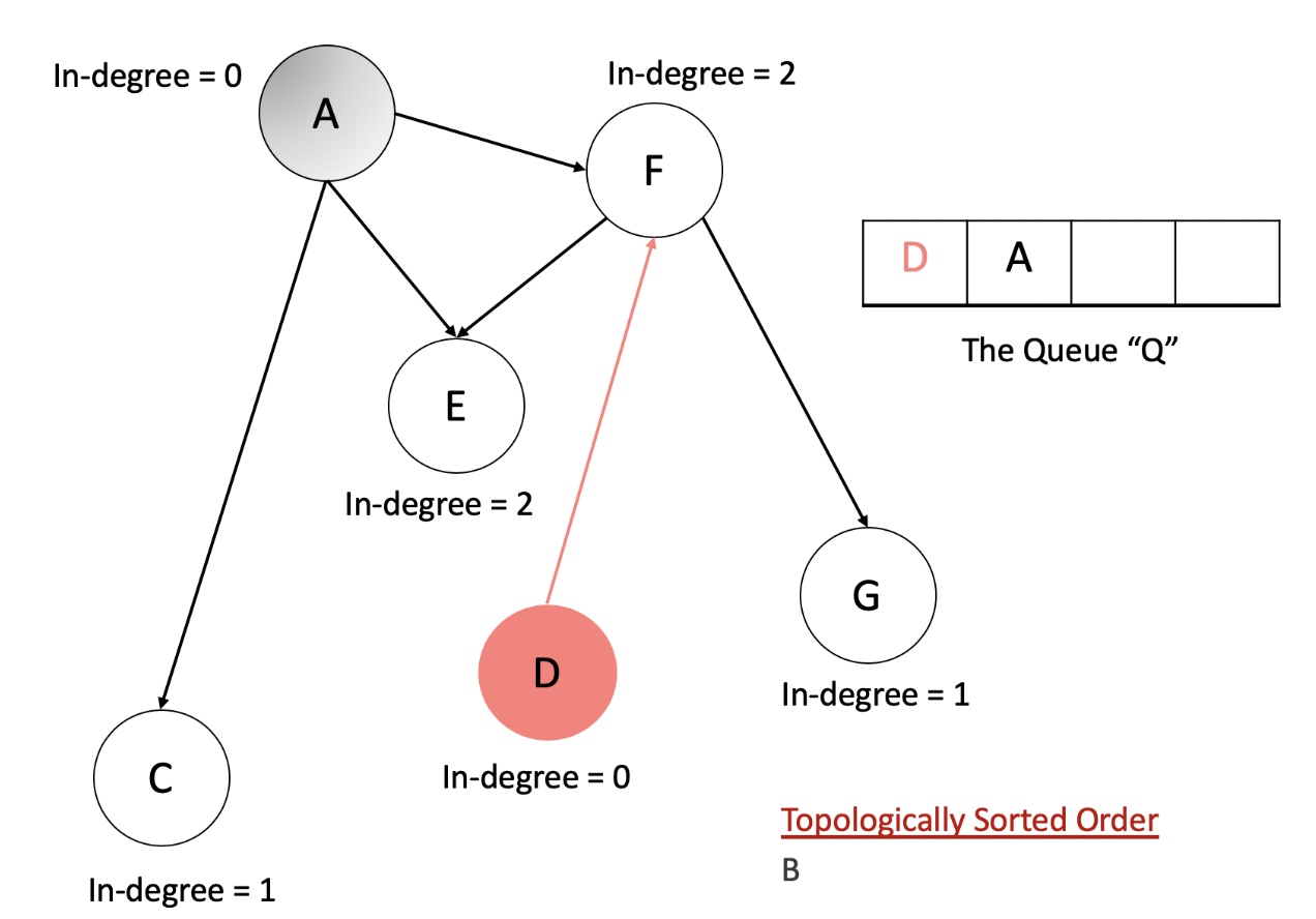
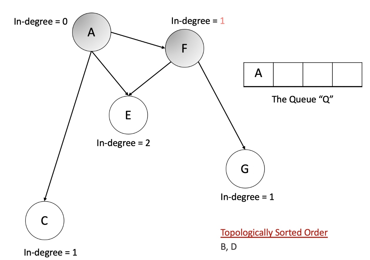
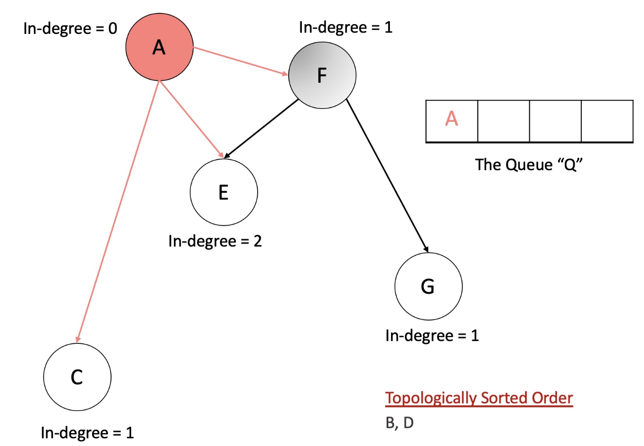
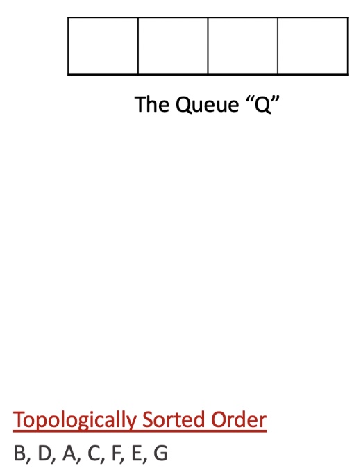
- Let’s look at an animated dry run of the algorithm on a sample graph before moving onto the formal implementations.
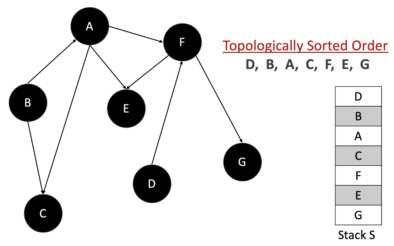
An important thing to note about topologically sorted order is that there won’t be just one ordering of nodes (courses). There can be multiple. For e.g. in the above graph, we could have processed the node “D” before we did “B” and hence have a different ordering.
from collections import defaultdict
class Solution:

    WHITE = 1
    GRAY = 2
    BLACK = 3

    def findOrder(self, numCourses, prerequisites):
        """
        :type numCourses: int
        :type prerequisites: List[List[int]]
        :rtype: List[int]
        """

        # Create the adjacency list representation of the graph
        adj_list = defaultdict(list)

        # A pair [a, b] in the input represents edge from b --> a
        for dest, src in prerequisites:
            adj_list[src].append(dest)

        topological_sorted_order = []
        is_possible = True

        # By default all vertces are WHITE
        color = {k: Solution.WHITE for k in range(numCourses)}
        def dfs(node):
            nonlocal is_possible

            # Don't recurse further if we found a cycle already
            if not is_possible:
                return

            # Start the recursion
            color[node] = Solution.GRAY

            # Traverse on neighboring vertices
            if node in adj_list:
                for neighbor in adj_list[node]:
                    if color[neighbor] == Solution.WHITE:
                        dfs(neighbor)
                    elif color[neighbor] == Solution.GRAY:
                         # An edge to a GRAY vertex represents a cycle
                        is_possible = False

            # Recursion ends. We mark it as black
            color[node] = Solution.BLACK
            topological_sorted_order.append(node)

        for vertex in range(numCourses):
            # If the node is unprocessed, then call dfs on it.
            if color[vertex] == Solution.WHITE:
                dfs(vertex)

        return topological_sorted_order[::-1] if is_possible else []
Complexity
-
Time: \(O(V + E)\) where \(V\) represents the number of vertices and \(E\) represents the number of edges. Essentially we iterate through each node and each vertex in the graph once and only once.
-
Space: \(O(V + E)\).
- We use the adjacency list to represent our graph initially. The space occupied is defined by the number of edges because for each node as the key, we have all its adjacent nodes in the form of a list as the value. Hence, \(O(E)\).
- Additionally, we apply recursion in our algorithm, which in worst case will incur \(O(E)\) extra space in the function call stack.
- To sum up, the overall space complexity is \(O(V + E)\).
Solution: Using Node Indegree / Kahn’s Algorithm
- Intuition:
- This approach is much easier to think about intuitively as will be clear from the following point/fact about topological ordering.
The first node in the topological ordering will be the node that doesn’t have any incoming edges. Essentially, any node that has an in-degree of 0 can start the topologically sorted order. If there are multiple such nodes, their relative order doesn’t matter and they can appear in any order.
- Our current algorithm is based on this idea. We first process all the nodes/course with 0 in-degree implying no prerequisite courses required. If we remove all these courses from the graph, along with their outgoing edges, we can find out the courses/nodes that should be processed next. These would again be the nodes with 0 in-degree. We can continuously do this until all the courses have been accounted for.
- This approach is much easier to think about intuitively as will be clear from the following point/fact about topological ordering.
- Algorithm:
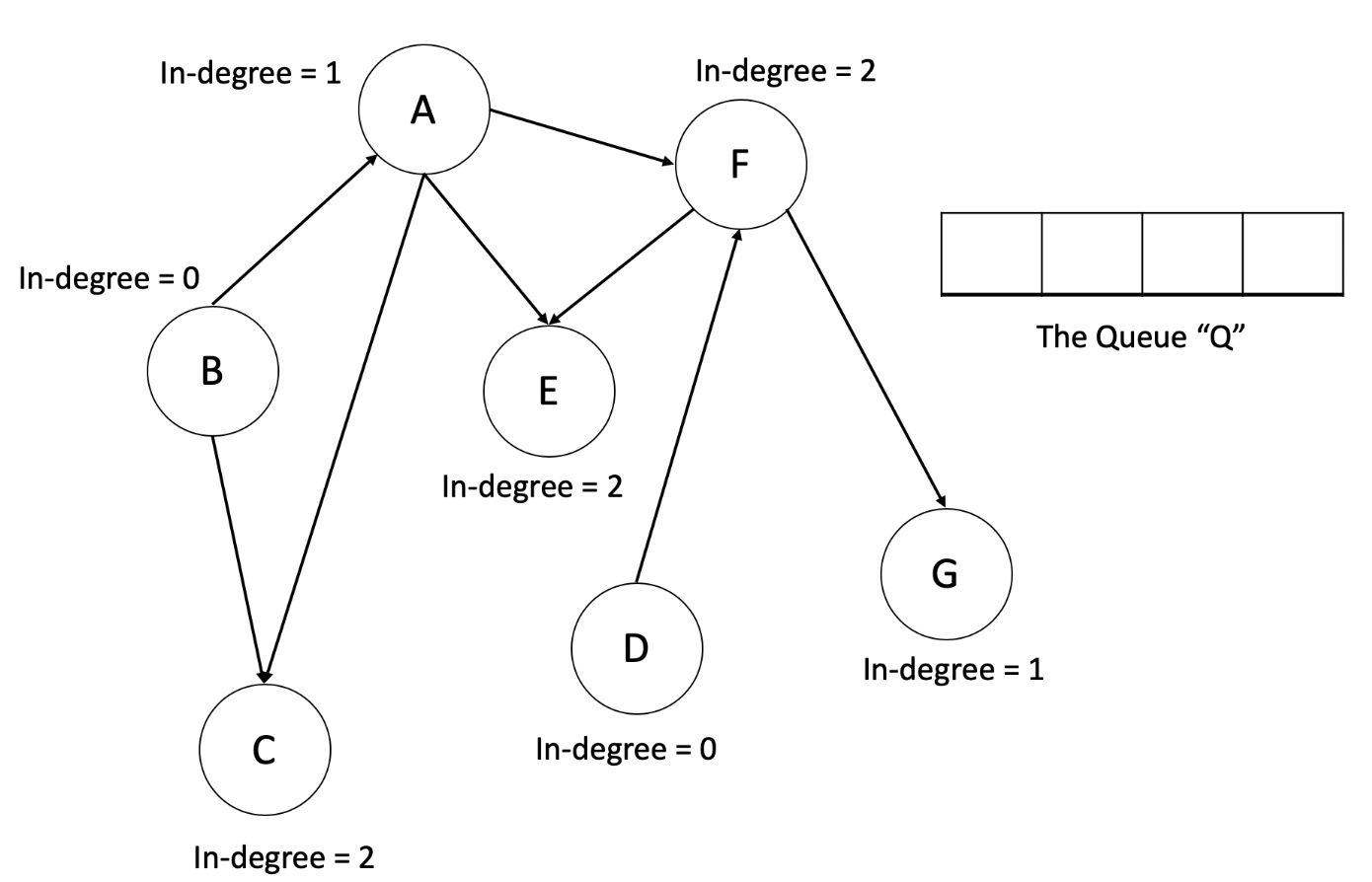
- Initialize a queue, Q to keep a track of all the nodes in the graph with 0 in-degree.
- Iterate over all the edges in the input and create an adjacency list and also a map of node v/s in-degree.
- Add all the nodes with 0 in-degree to
Q. - The following steps are to be done until the Q becomes empty.
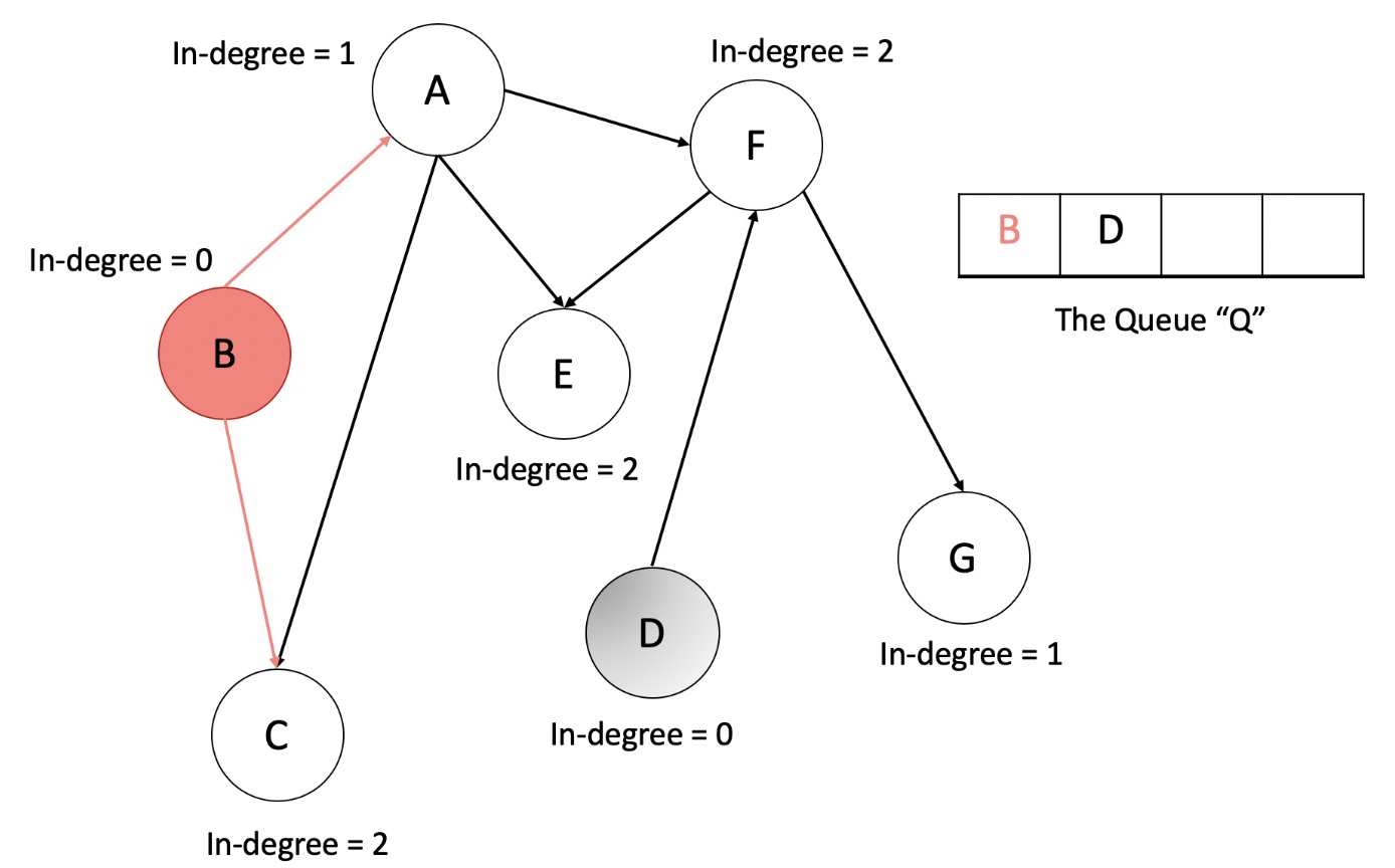
- Pop a node from the
Q. Let’s call this node,N. - For all the neighbors of this node,
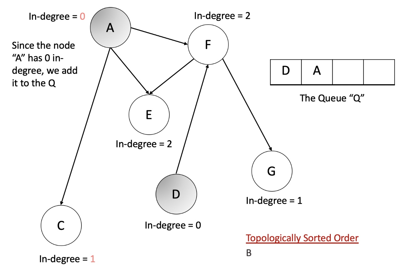
N, reduce their in-degree by 1. If any of the nodes’ in-degree reaches 0, add it to theQ. - Add the node N to the list maintaining topologically sorted order.
- Continue from step 4.1.
- Pop a node from the
- Let us now look at an animation depicting this algorithm and then we will get to the implementations.
- An important thing to note here is, using a queue is not a hard requirement for this algorithm. We can make use of a stack. That however, will give us a different ordering than what we might get from the queue because of the difference in access patterns between the two data-structures.
from collections import defaultdict, deque
class Solution:

    def findOrder(self, numCourses, prerequisites):
        """
        :type numCourses: int
        :type prerequisites: List[List[int]]
        :rtype: List[int]
        """

        # Prepare the graph
        adj_list = defaultdict(list)
        indegree = {}
        for dest, src in prerequisites:
            adj_list[src].append(dest)

            # Record each node's in-degree
            indegree[dest] = indegree.get(dest, 0) + 1

        # Queue for maintainig list of nodes that have 0 in-degree
        zero_indegree_queue = deque([k for k in range(numCourses) if k not in indegree])

        topological_sorted_order = []

        # Until there are nodes in the Q
        while zero_indegree_queue:

            # Pop one node with 0 in-degree
            vertex = zero_indegree_queue.popleft()
            topological_sorted_order.append(vertex)

            # Reduce in-degree for all the neighbors
            if vertex in adj_list:
                for neighbor in adj_list[vertex]:
                    indegree[neighbor] -= 1

                    # Add neighbor to Q if in-degree becomes 0
                    if indegree[neighbor] == 0:
                        zero_indegree_queue.append(neighbor)

        return topological_sorted_order if len(topological_sorted_order) == numCourses else []
Complexity
- Time: \(O(V + E)\) where \(V\) represents the number of vertices and \(E\) represents the number of edges. We pop each node exactly once from the zero in-degree queue and that gives us \(V\). Also, for each vertex, we iterate over its adjacency list and in totality, we iterate over all the edges in the graph which gives us \(E\). Hence, \(O(V + E)\).
- Space: \(O(V + E)\). We use an intermediate queue data structure to keep all the nodes with 0 in-degree. In the worst case, there won’t be any prerequisite relationship and the queue will contain all the vertices initially since all of them will have 0 in-degree. That gives us \(O(V)\). Additionally, we also use the adjacency list to represent our graph initially. The space occupied is defined by the number of edges because for each node as the key, we have all its adjacent nodes in the form of a list as the value. Hence, \(O(E)\). So, the overall space complexity is \(O(V + E)\).
[269/Hard] Alien Dictionary
Problem
-
There is a new alien language that uses the English alphabet. However, the order among the letters is unknown to you.
-
You are given a list of strings
wordsfrom the alien language’s dictionary, where the strings inwordsare sorted lexicographically by the rules of this new language. -
Return a string of the unique letters in the new alien language sorted in lexicographically increasing order by the new language’s rules. If there is no solution, return
"". If there are multiple solutions, return any of them. -
A string
sis lexicographically smaller than a string t if at the first letter where they differ, the letter inscomes before the letter intin the alien language. If the firstmin(s.length, t.length)letters are the same, then s is smaller if and only ifs.length < t.length. -
Example 1:
Input: words = ["wrt","wrf","er","ett","rftt"]
Output: "wertf"
- Example 2:
Input: words = ["z","x"]
Output: "zx"
- Example 3:
Input: words = ["z","x","z"]
Output: ""
Explanation: The order is invalid, so return "".
- Constraints:
1 <= words.length <= 1001 <= words[i].length <= 100words[i] consists of only lowercase English letters.
- See problem on LeetCode.
Solution: Topological sort with BFS (Kahn’s alogrithm)
- Overview:
- This explanation assumes you already have some confidence with graph algorithms, such as breadth-first search and depth-first searching. If you’re familiar with those, but not with topological sort (the topic tag for this problem), don’t panic, as you should still be able to make sense of it. It is one of the many more advanced algorithms that keen programmers tend to “invent” themselves before realizing it’s already a widely known and used algorithm. There are a couple of approaches to topological sort; Kahn’s Algorithm and DFS.
- A few things to keep in mind:
- The letters within a word don’t tell us anything about the relative order. For example, the presence of the word
kittenin the list does not tell us that the letterkis before the letteri. - The input can contain words followed by their prefix, for example,
abcdand thenab. These cases will never result in a valid alphabet (because in a valid alphabet, prefixes are always first). - You’ll need to make sure your solution detects these cases correctly. - There can be more than one valid alphabet ordering. It is fine for your algorithm to return any one of them.
- Your output string must contain all unique letters that were within the input list, including those that could be in any position within the ordering. It should not contain any additional letters that were not in the input.
- The letters within a word don’t tell us anything about the relative order. For example, the presence of the word
- Approaches:
- All approaches break the problem into three steps.
- Extracting dependency rules from the input. For example “A must be before C”, “X must be before D”, or “E must be before B”.
- Putting the dependency rules into a graph with letters as nodes and dependencies as edges (an adjacency list is best).
- Topologically sorting the graph nodes.
- All approaches break the problem into three steps.
- Intuition:
- There are three parts to this problem.
- Getting as much information about the alphabet order as we can out of the input word list.
- Representing that information in a meaningful way.
- Assembling a valid alphabet ordering.
- Part 1: Extracting Information:
- Let’s start with a large example of a dictionary in an “alien language”, and see how much we can conclude with some simple reasoning. This is likely to be your first step in tackling this question in a programming interview.
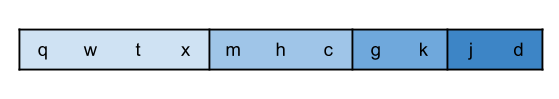
- Remember that in an ordinary English dictionary, all the words starting with a are at the start, followed by all the ones starting with
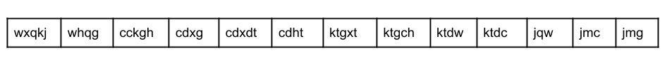
b, thenc,d,e, and at the very end,z. In the “alien dictionary”, we also expect the first letters of each word to be in alphabetical order. So, let’s look at them:[w, w, c, c, c, c, k, k, k, k, j, j]. - Removing the duplicates, we get:
[w, c, k, j]. - Going by this, we know the relative order of four letters in the “alien dictionary”. However, we don’t know how these four letters fit in with the other seven letters, or even how those other seven letters fit in with each other. To get more information, we’ll need to look further.
- Going back to the English dictionary analogy, the word
abacuswill appear beforealgorithm. This is because when the first letter of two words is the same, we instead look at the second letter;band1in this case.bis before1in the alphabet. - Let’s take a closer look at the first two words of the “alien dictionary”;
wxqkjandwhgg. Seeing as the first letters are the same,w, we look at the second letters. The first word hasx, and the second word has $h$. Therefore, we know thatxis beforehin the alien dictionary. We know have two fragments of the letter-order:[w, c, k, j],[x, h]. - We don’t know yet how these two fragments could fit together into a single ordering. For example, we don’t know whether w is before x, or x is before w, or even whether or not there’s enough information available in the input for us to know.
- Anyway, we’ve now gotten all the information we can out of the first two words. All letters after
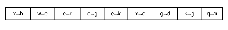
xinwxqkj, and afterhinwhqg, should be ignored because they did not impact the relative ordering of the two words (if you’re confused, think back toabacusandalgorithm. Becauseb > l, thegorithmandacusparts are unimportant for determining alphabetical ordering). - Hopefully, you’re starting to see a pattern here. Where two words are adjacent, we need to look for the first difference between them. That difference tells us the relative order between two letters. Let’s have a look at all the relations we can find by comparing adjacent words.
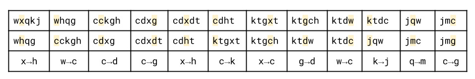
- You might notice that we haven’t included some rules, such as
w → j. This is fine though, as we can still derive it from the rules we have:w → c, c → k, k → j. - This completes the first part. There is no further information we can extract from the input. Therefore, our task is now to put together what we know.
- Let’s start with a large example of a dictionary in an “alien language”, and see how much we can conclude with some simple reasoning. This is likely to be your first step in tackling this question in a programming interview.
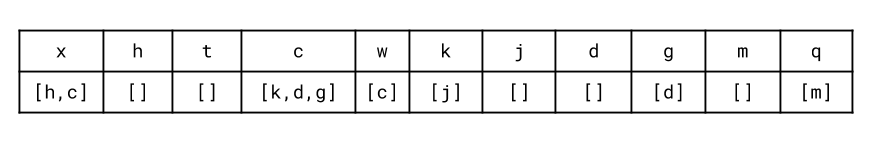
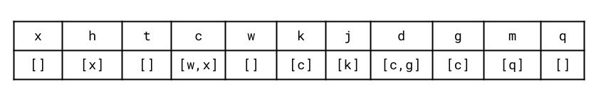
- Part 2: Representing the Relations:
- We now have a set of relations stating how pairs of letters are ordered relative to each other.
- How could we put these together? You may be tempted to start trying to build “chains” out of them. Here are a few possible chains.
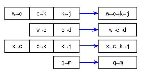
- The problem here though is that some letters are in more than one chain. Simply putting the chains into the output list one-after-the-other won’t work. Some letters will be duplicated, which invalidates the ordering. Simply deleting the duplicates will not work either.
- When we have a set of relations, often drawing a graph is the best way to visualize them. The nodes are the letters, and an edge between two letters,
AandBrepresents thatAis beforeBin the “alien alphabet”.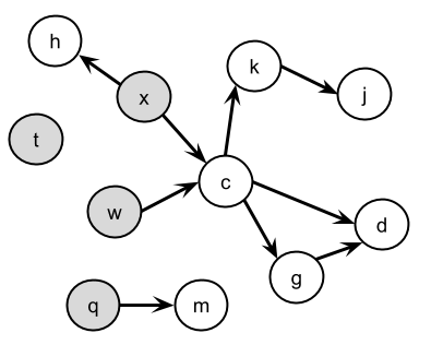
- We now have a set of relations stating how pairs of letters are ordered relative to each other.
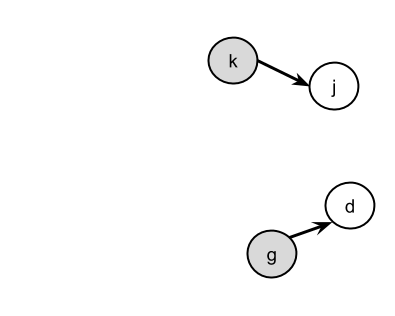
- Part 3: Assembling a Valid Ordering:
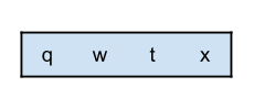
- As we can see from the graph, four of the letters have no arrows going into them. What this means is that there are no letters that have to be before any of these four (remember that the question states there could be multiple valid orderings, and if there are, then it’s fine for us to return any of them).
- Therefore, a valid start to the ordering we return would be:
- We can now remove these letters and edges from the graph, because any other letters that required them first will now have this requirement satisfied.
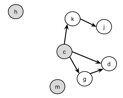
- On this new graph, there are now three new letters that have no in-arrows. We can add these to our output list.
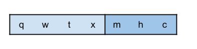
- Again, we can remove these from the graph.
- Then add the two new letters with no in-arrows.

- Which leaves the following graph.
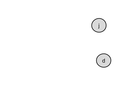
- With the final two letters.
- Which is a valid ordering that we can return.
- As a side note, each of the four groups of letters we picked off could have been in any order within themselves (as another side note, it’s not too difficult to calculate how many valid orderings there are. Have a think about this if you want, determining how many valid alphabet orderings there are is an interesting follow-up question!)
- There are three parts to this problem.
- Algorithm:
- Now that we have come up with an approach, we need to figure out how to implement it efficiently.
- The first and second parts are straightforward; we’ll leave you to look at the code for these. It should extract the order relations and then insert them into an adjacency list. The only thing we need to be careful of is ensuring that we’ve handled the “prefix” edge case correctly.
- The third part is more complicated. We need to somehow identify which letters have no incoming links left. With the adjacency list format above, this is a bit annoying to do, because determining whether or not a particular letter has any incoming links requires repeatedly checking over the adjacency lists of all the other letters to see whether or not they feature that letter.
- A naïve solution would be to do exactly this. While this would be efficient enough with at most 26 letters, it may result in your interviewer quickly telling you that we might want to use the same algorithm on an “alien language” with millions of unique letters.
- An alternative is to keep two adjacency lists; one the same as above, and another that is the reverse, showing the incoming links. Then, each time we traverse an edge, we could remove the corresponding edge in the reverse adjacency list. Seeing when a letter has no more incoming links would now be straightforward.
- However, we can do even better than that. Instead of keeping track of all the other letters that must be before a particular letter, we only need to keep track of how many of them there are! While building the forward adjacency list, we can also count up how many incoming edges each letter has. We call the number of incoming edges the indegree of a node.
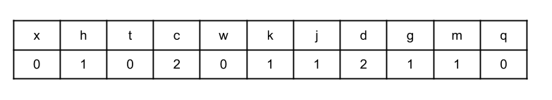
- Then, instead of removing an edge from a reverse adjacency list, we can simply decrement the count by 1. Once the count reaches 0, this is equivalent to there being no incoming edges left in the reverse adjacency list.
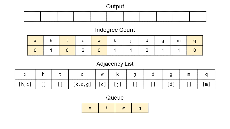
- We’ll do a BFS for all letters that are reachable, adding each letter to the output as soon as it’s reachable. A letter is reachable once all of the letters that need to be before it have been added to the output. To do a BFS, recall that we use a queue. We should initially put all letters with an in-degree of 0 onto that queue. Each time a letter gets down to an in-degree of 0, it is added to the queue.
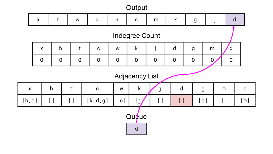
- We continue this until the queue is empty. After that, we check whether or not all letters were put in the output list. If some are missing, this is because we got to a point where all remaining letters had at least one edge going in; this means there must be a cycle! In that case, we should return “” as per the problem description. Otherwise, we should return the complete ordering we found.
- One edge case we need to be careful of is where a word is followed by its own prefix. In these cases, it is impossible to come up with a valid ordering and so we should return “”. The best place to detect it is in the loop that compares each adjacent pair of words.
- Also, remember that not all letters will necessarily have an edge going into or out of them. These letters can go anywhere in the output. But we need to be careful to not forget about them in our implementation.
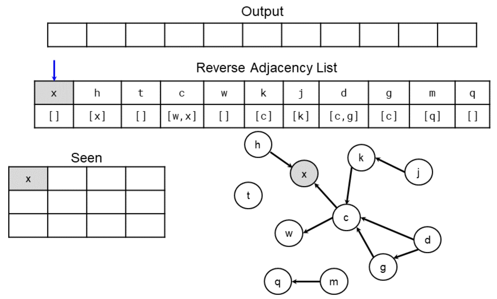
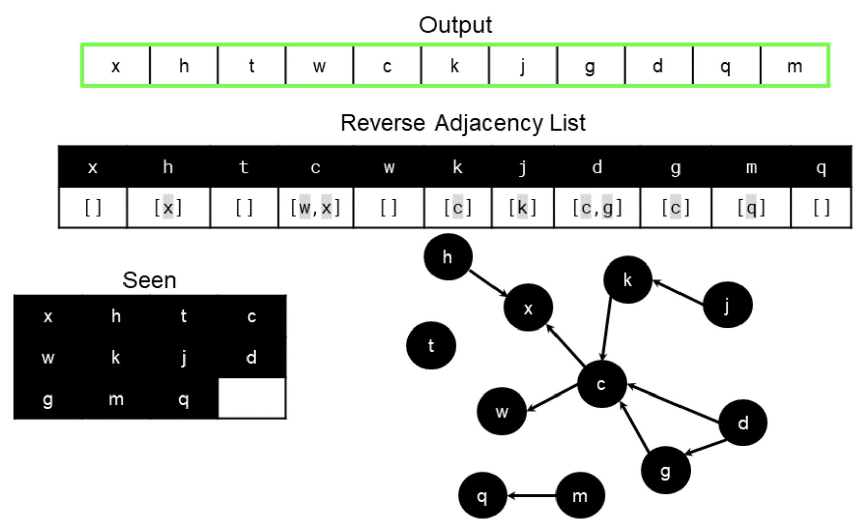
- Here are diagrams showing the entire algorithm on our example from earlier. The first image shows the start while the second shows the end.
from collections import defaultdict, Counter, deque

class Solution:
    def alienOrder(self, words: List[str]) -> str:
        # Step 0: create data structures + the in_degree of each unique letter to 0.
        adj_list = defaultdict(set)
        in_degree = Counter({c : 0 for word in words for c in word})

        # Step 1: We need to populate adj_list and in_degree.
        # For each pair of adjacent words...
        for first_word, second_word in zip(words, words[1:]):
            for c, d in zip(first_word, second_word):
                if c != d:
                    if d not in adj_list[c]:
                        adj_list[c].add(d)
                        in_degree[d] += 1
                    break
            else: # Check that second word isn't a prefix of first word.
                if len(second_word) < len(first_word): return ""

        # Step 2: We need to repeatedly pick off nodes with an indegree of 0.
        output = []
        queue = deque([c for c in in_degree if in_degree[c] == 0])
        while queue:
            c = queue.popleft()
            output.append(c)
            for d in adj_list[c]:
                in_degree[d] -= 1
                if in_degree[d] == 0:
                    queue.append(d)

        # If not all letters are in output, that means there was a cycle and so
        # no valid ordering. Return "" as per the problem description.
        if len(output) < len(in_degree):
            return ""
        # Otherwise, convert the ordering we found into a string and return it.
        return "".join(output)
- Similar approach; rehashed:
- Preparation steps:
- Calculate all edges by comparing adjacent words, and then compare each letter between two words until equality fails at some letter. E.g. compare
"wrt"and"wrf", the output edge will be:'t' -> 'f'. Here we can say,'f'depends on't'. - Calculate in degrees (init is zero) for each vertex by traversing all edges above. E.g. for edge ‘t’ -> ‘f’ above, in degrees of ‘f’ should be added 1 while in degrees of ‘t’ stays the same.
- Picking all the vertices with zero in degree. We can get all vertices by python’s set by concatenating all words:
set(''.join(words)).
- Calculate all edges by comparing adjacent words, and then compare each letter between two words until equality fails at some letter. E.g. compare
- Preparation steps:
from typing import List
from collections import defaultdict

class Solution:
    def alienOrder(self, words: List[str]) -> str:
        # calculate all edges (u->v, in which u must be ahead of v in alien dictionary)
        edges = defaultdict(set)
        degrees = defaultdict(int)

        for two_words in zip(words, words[1:]): # compare adjacent words
            for ch1, ch2 in zip(*two_words): # compare letter by letter between two words
                if ch1 != ch2: # ch1 -> ch2 (degree[ch2]++)
                    edges[ch1].add(ch2) # ch2 depends on (is after) ch1
                    break

        # calculate in-degrees for all vertices
        for ch in edges.keys():
            for ch2 in edges[ch]:
                degrees[ch2] += 1

        charset = set(''.join(words)) # get all vertices
        q = [ch for ch in charset if ch not in degrees] # degree=0 as start nodes
        res = []

        while q:
            ch = q.pop(0)
            res.append(ch)
            for ch2 in edges[ch]:
                degrees[ch2] -= 1
                if degrees[ch2] == 0:
                    q.append(ch2)

        if all(map(lambda d: d==0, degrees.values())): # all vertex in degrees are zero, acyclic graphs
            return ''.join(res)

        return '' # otherwise, circle found in graph
Complexity
- Let \(N\) be the total number of strings in the input list, \(C\) be the total length of all the words in the input list added together, \(U\) be the total number of unique letters in the alien alphabet. While this is limited to 26 in the question description, we’ll still look at how it would impact the complexity if it was not limited (as this could potentially be a follow-up question).
- Time: \(O(C)\)
- There were three parts to the algorithm; identifying all the relations, putting them into an adjacency list, and then converting it into a valid alphabet ordering.
- In the worst case, the first and second parts require checking every letter of every word (if the difference between two words was always in the last letter). This is \(O(C)\).
- For the third part, recall that a breadth-first search has a cost of \(O(V + E)\), where \(V\) is the number of vertices and EE is the number of edges. Our algorithm has the same cost as BFS, as it too is visiting each edge and node once (a node is visited once all of its edges are visited, unlike the traditional BFS where it is visited once one edge is visited). Therefore, determining the cost of our algorithm requires determining how many nodes and edges there are in the graph.
- Nodes: We know that there is one vertex for each unique letter, i.e. \(O(U)\) vertices.
- Edges: Each edge in the graph was generated from comparing two adjacent words in the input list. There are \(N - 1\) pairs of adjacent words, and only one edge can be generated from each pair. This might initially seem a bit surprising, so let’s quickly look at an example. We’ll use English words.
abacus algorithm - The only conclusion we can draw is that b is before l. This is the reason abacus appears before algorithm in an English dictionary. The characters afterward are irrelevant. It is the same for the “alien” alphabets we’re working with here. The only rule we can draw is the one based on the first difference between the two words.
- Also, remember that we are only generating rules for adjacent words. We are not adding the “implied” rules to the adjacency list. For example, assume we have the following word list.
rgh xcd tny bcd - We are only generating the following 3 edges.
r -> x x -> t t -> b - We are not generating these implied rules (the graph structure shows them indirectly).
r -> t r -> b x -> b - So with this, we know that there are at most \(N - 1\) edges.
- There is an additional upper limit on the number of edges too—it is impossible for there to be more than one edge between each pair of nodes. With \(U\) nodes, this means there can’t be more than \(U^2\) edges.
- It’s not common in complexity analysis that we get two separate upper bounds like this. Because the number of edges has to be lower than both \(N - 1\) and \(U^2\), we know it is at most the smallest of these two values. Mathematically, we can say this is \(\min(U^2, N - 1)\).
- Going all the way back to the cost of breadth first search, we can now substitute in the number of nodes and the number of edges: \(V = U\) and \(E = \min(U^2, N - 1)\). This gives us: \(O(V + E) = O(U + \min(U^2, N - 1)) = O(U + \min(U^2, N))\)
- Finally, we need to combine the two parts: \(O(C)\) for the first and second parts, and \(O(U + \min(U^2, N))\) for the third part. When we have two independent parts, we add the costs together, as we don’t necessarily know which is larger. After we’ve done this, we should look at the final formula and see whether or not we can actually draw any conclusions about which is larger. Adding them together, we initially get the following: \(O(C) + O(U + \min(U^2, N)) = O(C + U + \min(U^2, N))\)
- So, what do we know about the relative values of \(N\), \(C\), and \(U\)? Well, we know that \(N < C\), as each word contains at least one character (remember, \(C\) is total characters across the words, not unique characters). Additionally, \(U < C\) because there can’t be more unique characters than there are characters.
- In summary, CC is the biggest of the three, and NN and UU are smaller, although we don’t know which is smaller out of those two.
- So for starters, we know that the UU bit is insignificant compared to the CC. Therefore, we can just remove it: \(O(C + U + \min(U^2, N)) → O(C + \min(U^2, N))\)
- Now, to simplify the rest, consider two cases:
- If \(U^2\) is smaller than \(N\), then \(\min(U^2, N) = U^2\). By definition, we’ve just said that \(U^2\) is smaller than \(N\), which is in turn smaller than \(C\), and so \(U^2\) is definitely less than \(C\). This leaves us with \(O(C)\).
- If \(U^2\) is larger than \(N\), then \(\min(U^2, N) = N\). Because \(C > N\), we’re left with \(O(C)\).
- So in all cases, we know that \(C > \min(U^2, N)\). This gives us a final time complexity of \(O(C)\).
- Space: \(O(1)\) or \(O(U + \min(U^2, N))\)
- The adjacency list uses the most auxiliary memory. This list uses \(O(V + E)\) memory, where \(V\) is the number of unique letters, and \(E\) is the number of relations.
- The number of vertices is simply \(U\); the number of unique letters.
- The number of edges in the worst case is \(\min(U^2, N)\), as explained in the time complexity analysis.
- So in total the adjacency list takes \(O(U + \min(U^2, N))\) space.
- So for the question we’re given, where UU is a constant fixed at a maximum of 26, the space complexity is simply \(O(1)\). This is because \(U\) is fixed at 26, and the number of relations is fixed at \(26^2\), so \(O(\min(26^2, N)) = O(26^2) = O(1)\).
- But when we consider an arbitrarily large number of possible letters, we use the size of the adjacency list; \(O(U + \min(U^2, N))\).
Solution: Topological sort without BFS
- We do not need a DFS or BFS to detect if there is a cycle, because if the graph stops shrinking before all nodes are removed, it indicates that solution doesn’t exist (a cycle in the graph).
class Node(object):
    def __init__(self):
        self.IN = set()
        self.OUT = set()

class Solution:
    def alienOrder(self, words: List[str]) -> str:
        # initialization
        allnodes, graph, res = set("".join(words)), {}, ""
        for i in allnodes:
            graph[i] = Node()

        # build the graph
        for i in range(len(words)-1):
            # obey lexicographical sorting rule
            if words[i].find(words[i + 1]) == 0 and len(words[i]) > len(words[i + 1]):
                return ""

            for j in zip(words[i], words[i+1]):
                if j[0] != j[1]:
                    graph[j[0]].OUT.add(j[1])
                    graph[j[1]].IN.add(j[0])
                    break

        # topo-sort
        while allnodes:
            buff = set([i for i in allnodes if graph[i].OUT and not graph[i].IN])
            if not buff:
                return res + "".join(allnodes) if not [i for i in allnodes if graph[i].IN] else "" # have solution if no connected node
            res += "".join(buff)
            allnodes -= buff
            for i in allnodes:
                graph[i].IN -= buff
        return res
Complexity
- Time: \(O(C)\)
- Building the adjacency list has a time complexity of \(O(C)\) for the same reason as in the BFS approach.
- Again, like in the BFS approach, we traverse every “edge”, but this time we’re using depth-first-search.
- Space: \(O(1)\) or \(O(U + \min(U^2, N))\)
- Like in the BFS approach, we build an adjacency list. Even though this one is a reversed adjacency list, it still contains the same number of relations.
Solution: DFS
- Intuition:
- Another approach to the third part is to use a depth-first search. We still need to extract relations and then generate an adjacency list in the same way as before, but this time we don’t need the
indegreesmap. - Recall that in a depth-first search, nodes are returned once they either have no outgoing links left, or all their outgoing links have been visited. Therefore, the order in which nodes are returned by the depth-first search will be the reverse of a valid alphabet order.
- Another approach to the third part is to use a depth-first search. We still need to extract relations and then generate an adjacency list in the same way as before, but this time we don’t need the
- Algorithm:
- If we made a reverse adjacency list instead of a forward one, the output order would be correct (without needing to be reversed). Remember that when we reverse the edges of a directed graph, the nodes with no incoming edges became the ones with no outgoing edges. This means that the ones at the start of the alphabet will now be the ones returned first.
- One issue we need to be careful of is cycles. In directed graphs, we often detect cycles by using graph coloring. All nodes start as white, and then once they’re first visited they become grey, and then once all their outgoing nodes have been fully explored, they become black. We know there is a cycle if we enter a node that is currently grey (it works because all nodes that are currently on the stack are grey. Nodes are changed to black when they are removed from the stack).
- Here are a set of diagrams showing the DFS, starting from a reverse adjacency list of the input. The first one shows the initial step, while the second one shows the final step.
from collections import defaultdict, Counter, deque

class Solution:
    def alienOrder(self, words: List[str]) -> str:

        # Step 0: Put all unique letters into the adj list.
        reverse_adj_list = {c : [] for word in words for c in word}

        # Step 1: Find all edges and put them in reverse_adj_list.
        for first_word, second_word in zip(words, words[1:]):
            for c, d in zip(first_word, second_word):
                if c != d:
                    reverse_adj_list[d].append(c)
                    break
            else: # Check that second word isn't a prefix of first word.
                if len(second_word) < len(first_word):
                    return ""

        # Step 2: Depth-first search.
        seen = {} # False = grey, True = black.
        output = []
        def visit(node):  # Return True iff there are no cycles.
            if node in seen:
                return seen[node] # If this node was grey (False), a cycle was detected.
            seen[node] = False # Mark node as grey.
            for next_node in reverse_adj_list[node]:
                result = visit(next_node)
                if not result:
                    return False # Cycle was detected lower down.
            seen[node] = True # Mark node as black.
            output.append(node)
            return True

        if not all(visit(node) for node in reverse_adj_list):
            return ""

        return "".join(output)
Complexity
- Time: \(O(C)\)
- Building the adjacency list has a time complexity of \(O(C)\) for the same reason as in the BFS approach.
- Again, like in the BFS approach, we traverse every “edge”, but this time we’re using depth-first-search.
- Space: \(O(1)\) or \(O(U + \min(U^2, N))\)
- Like in the BFS approach, we build an adjacency list. Even though this one is a reversed adjacency list, it still contains the same number of relations.
[444/Medium] Sequence Reconstruction
Problem
-
You are given an integer array
numsof length n wherenumsis a permutation of the integers in the range[1, n]. You are also given a 2D integer array sequences wheresequences[i]is a subsequence ofnums. -
Check if
numsis the shortest possible and the only supersequence. The shortest supersequence is a sequence with the shortest length and has allsequences[i]as subsequences. There could be multiple valid supersequences for the given array sequences.- For example, for
sequences = [[1,2],[1,3]], there are two shortest supersequences,[1,2,3]and[1,3,2]. - While for
sequences = [[1,2],[1,3],[1,2,3]], the only shortest supersequence possible is[1,2,3].[1,2,3,4]is a possible supersequence but not the shortest.
- For example, for
-
Return true if
numsis the only shortest supersequence for sequences, or false otherwise. -
A subsequence is a sequence that can be derived from another sequence by deleting some or no elements without changing the order of the remaining elements.
-
Example 1:
Input: nums = [1,2,3], sequences = [[1,2],[1,3]]
Output: false
Explanation: There are two possible supersequences: [1,2,3] and [1,3,2].
The sequence [1,2] is a subsequence of both: [1,2,3] and [1,3,2].
The sequence [1,3] is a subsequence of both: [1,2,3] and [1,3,2].
Since nums is not the only shortest supersequence, we return false.
- Example 2:
Input: nums = [1,2,3], sequences = [[1,2]]
Output: false
Explanation: The shortest possible supersequence is [1,2].
The sequence [1,2] is a subsequence of it: [1,2].
Since nums is not the shortest supersequence, we return false.
- Example 3:
Input: nums = [1,2,3], sequences = [[1,2],[1,3],[2,3]]
Output: true
Explanation: The shortest possible supersequence is [1,2,3].
The sequence [1,2] is a subsequence of it: [1,2,3].
The sequence [1,3] is a subsequence of it: [1,2,3].
The sequence [2,3] is a subsequence of it: [1,2,3].
Since nums is the only shortest supersequence, we return true.
- Constraints:
n == nums.length1 <= n <= 104nums is a permutation of all the integers in the range [1, n].1 <= sequences.length <= 1041 <= sequences[i].length <= 1041 <= sum(sequences[i].length) <= 1051 <= sequences[i][j] <= nAll the arrays of sequences are unique.sequences[i] is a subsequence of nums.
- See problem on LeetCode.
Solution: Topological Sort
from collections import deque

class Solution(object):
    def sequenceReconstruction(self, org, seqs):
        """
        :type org: List[int]
        :type seqs: List[List[int]]
        :rtype: bool
        """
        sortedOrder = []
        if len(org) <= 0:
            return False

        # a. Initialize the graph
        inDegree = {}                                       # count of incoming edges
        graph = {}                                          # adjacency list graph
        for seq in seqs:
            for num in seq:
                inDegree[num] = 0
                graph[num] = []

        # b. Build the graph
        for seq in seqs:
            for idx in range(0, len(seq) - 1):
                parent, child = seq[idx], seq[idx + 1]
                graph[parent].append(child)
                inDegree[child] += 1

        # if we don't have ordering rules for all the numbers we'll not able to uniquely construct the sequence
        if len(inDegree) != len(org):
            return False

        # c. Find all sources i.e., all vertices with 0 in-degrees
        sources = deque()
        for key in inDegree:
            if inDegree[key] == 0:
                sources.append(key)

        # d. For each source, add it to the sortedOrder and subtract one from all of its children's in-degrees
        # if a child's in-degree becomes zero, add it to the sources queue
        while sources:
            if len(sources) > 1:
                return False                                # more than one sources mean, there is more than one way to reconstruct the sequence
            if org[len(sortedOrder)] != sources[0]:
                return False                                # the next source(or number) is different from the original sequence

            vertex = sources.popleft()
            sortedOrder.append(vertex)
            for child in graph[vertex]:                     # get the node's children to decrement their in-degrees
                inDegree[child] -= 1
                if inDegree[child] == 0:
                    sources.append(child)

        # if sortedOrder's size is not equal to original sequence's size, there is no unique way to construct
        return len(sortedOrder) == len(org)
Complexity
- Time: \(O(\midV\mid+\midE\mid)\)
- Space: \(O(\midV\mid+\midE\mid)\)
[1203/Hard] Sort Items by Groups Respecting Dependencies
Problem
- There are
nitems each belonging to zero or one of m groups where group[i] is the group that the i-th item belongs to and it’s equal to -1 if the i-th item belongs to no group. The items and the groups are zero indexed. A group can have no item belonging to it. -
Return a sorted list of the items such that:
- The items that belong to the same group are next to each other in the sorted list.
- There are some relations between these items where beforeItems[i] is a list containing all the items that should come before the i-th item in the sorted array (to the left of the i-th item).
- Return any solution if there is more than one solution and return an empty list if there is no solution.
- Example 1:
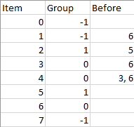
Input: n = 8, m = 2, group = [-1,-1,1,0,0,1,0,-1], beforeItems = [[],[6],[5],[6],[3,6],[],[],[]]
Output: [6,3,4,1,5,2,0,7]
- Example 2:
Input: n = 8, m = 2, group = [-1,-1,1,0,0,1,0,-1], beforeItems = [[],[6],[5],[6],[3],[],[4],[]]
Output: []
Explanation: This is the same as example 1 except that 4 needs to be before 6 in the sorted list.
- Constraints:
1 <= m <= n <= 3 * 104group.length == beforeItems.length == n-1 <= group[i] <= m - 10 <= beforeItems[i].length <= n - 10 <= beforeItems[i][j] <= n - 1i != beforeItems[i][j]beforeItems[i] does not contain duplicates elements.
- See problem on LeetCode.
Solution: 2-Level Topological Sort using DFS
- The basic idea is to split the problem into two parts and to do a two-level topological sort (one for each part). First on groups, then on items. Topological sort is done using DFS with a stack for cycle detection.
from collections import defaultdict
from collections.abc import Iterable

class Solution:
    def sortItems(self, n: int, m: int, group: List[int], beforeItems: List[List[int]]) -> List[int]:
        # add missing groups
        for i in range(n):
            if group[i] == -1:
                group[i], m = m, m+1

        # translate beforeItems to group dependencies
        group_deps = [set() for _ in range(m)]
        for i in range(n):
            for j in beforeItems[i]:
                # don't add own group as a dependency
                if group[i] != group[j]:
                    group_deps[group[i]].add(group[j])

        def topo_order(deps: list[Iterable[int]]):
            order = []
            visited = set()
            stack = set()
            def dfs(i):  # return True if cycle detected
                if i in stack:
                    return True
                if i in visited:
                    return False
                visited.add(i)
                stack.add(i)
                for dep in deps[i]:
                    if dfs(dep):
                        return True
                # topological ordering is post-order DFS
                order.append(i)
                stack.remove(i)
            for i in range(len(deps)):
                if dfs(i):
                    return None  # if cycle detected return None
            return order

        group_order = topo_order(group_deps)
        item_order = topo_order(beforeItems)
        # if a cycle is detected in groups or items, return []
        if group_order is None or item_order is None:
            return []
        # regroup items by group num
        group_items = defaultdict(list)
        for i in item_order:
            group_items[group[i]].append(i)
        return [i for g in group_order for i in group_items[g]]
Solution: 1-Level Topological Sort
- Key takeaways:
- Some elements belong to no group.
- The
beforeItemsarray is given for each element that denotes the elements that have to come before this. - Elements that are in the same group need to come together.
- First easy solution:
- Assign auto increasing groups to ones that have no group (-1)
- Perform topological sort on all the groups
- Perform topological sort within each group
- The above solution works but is apparently not elegant so we come up with a new one.
- In this new solution, we add 2 extra nodes per group. A start and end node. Idea is that we connect start and all nodes of a group with a directed edge. We connect all nodes and the end with a directed edge.
- If two nodes are among different groups in the
beforeItems, we connect the endNode of first group with the startNode of the second group. - Notice that we rewire all intergroup connections between these nodes alone. Essentially, this will ensure that all nodes in a particular group are done and only then the other group starts (as we introduced edge from the endNode and startNode this is guaranteed).
- By property of topological sort, when we do this, we force all nodes in the same group to appear together in the end result.
- Important:
- Notice we do separate topological sort operations on all the initial start nodes then concatenate. This is essential for this problem to ensure other island nodes do not pop up in the current group.
class Solution:
    def sortItems(self, n: int, m: int, group: List[int], beforeItems: List[List[int]]) -> List[int]:
        beforeNodes = [n + 2 * i for i in range(m)]  # these are the starting nodes for a group
        afterNodes = [n + 2 * i + 1 for i in range(m)]  # these are the ending nodes for a group
        nodeSet = []
        graph = defaultdict(list)
        in_degree = defaultdict(int)
        for i, (group_id, before_list) in enumerate(zip(group, beforeItems)):
            nodeSet.append(i)
            if group_id != -1:
                graph[beforeNodes[group_id]].append(i)  # adding directed edge from before node to this node
                graph[i].append(afterNodes[group_id])  # adding directed edge from current node to after node
                in_degree[i] += 1
                in_degree[afterNodes[group_id]] += 1

            for node in before_list:
                # different cases for connection. read properly
                if group[i] == group[node]:
                    graph[node].append(i)
                    in_degree[i] += 1
                elif group[i] == -1:
                    if group[node] == -1:
                        graph[node].append(i)
                    else:
                        graph[afterNodes[group[node]]].append(i)
                    in_degree[i] += 1
                else:
                    if group[node] == -1:
                        graph[node].append(beforeNodes[group[i]])
                    else:
                        graph[afterNodes[group[node]]].append(beforeNodes[group[i]])
                    in_degree[beforeNodes[group[i]]] += 1

        starts = deque()
        for node in nodeSet + beforeNodes + afterNodes:
            if not in_degree[node]:
                starts.append(node)

        res = []
        for s in starts:
            temp_res = []
            sources = deque([s])
            while sources:
                cur = sources.popleft()
                temp_res.append(cur)

                for node in graph[cur]:
                    in_degree[node] -= 1
                    if not in_degree[node]:
                        sources.append(node)
            res += temp_res

        res = [x for x in res if x < n]

        if len(res) != n:
            return []

        return res
Complexity
- Time: \(O(\midV\mid+\midE\mid)\)
- Space: \(O(\midV\mid+\midE\mid)\)