Distilled • LeetCode • Sorting/Searching
- Pattern: Sorting/Searching
- [148/Medium] Sort List
- Problem
- Solution: QuickSort
- Solution: Insertion Sort
- Solution: Top Down/Recursive Merge Sort; recursively split the list into two parts, merge the two resulting sorted lists
- Solution: Bottom Up/Iterative Merge Sort (better space complexity); recursively split the list into two parts, merge the two resulting sorted lists
- [912/Medium] Sort an Array
- [148/Medium] Sort List
Pattern: Sorting/Searching
[148/Medium] Sort List
Problem
-
Given the head of a linked list, return the list after sorting it in ascending order.
-
Example 1:
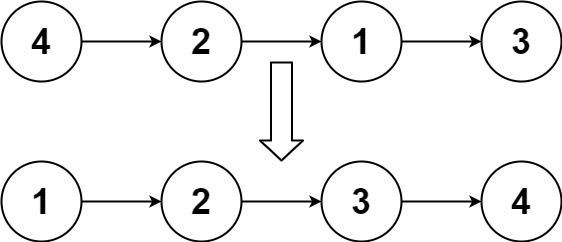
Input: head = [4,2,1,3]
Output: [1,2,3,4]
- Example 2:
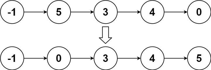
Input: head = [-1,5,3,4,0]
Output: [-1,0,3,4,5]
- Example 3:
Input: head = []
Output: []
- Constraints:
The number of nodes in the list is in the range [0, 5 * 104].-105 <= Node.val <= 105
-
Follow up: Can you sort the linked list in
O(n logn)time andO(1)memory (i.e. constant space)? - See problem on LeetCode.
Solution: QuickSort
- Algorithm:
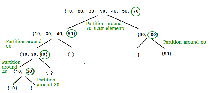
- Like Merge Sort, QuickSort is a Divide and Conquer algorithm. It picks an element as pivot and partitions the given array around the picked pivot. There are many different versions of quickSort that pick pivot in different ways.
- Always pick first element as pivot.
- Always pick last element as pivot (implemented below)
- Pick a random element as pivot.
- Pick median as pivot.
- The key process in quickSort is
partition(). Target of partitions is, given an array and an elementxof array as pivot, putxat its correct position in sorted array and put all smaller elements (smaller thanx) beforex, and put all greater elements (greater thanx) afterx. All this should be done in linear time.
- Like Merge Sort, QuickSort is a Divide and Conquer algorithm. It picks an element as pivot and partitions the given array around the picked pivot. There are many different versions of quickSort that pick pivot in different ways.
- Why Quick Sort is preferred over MergeSort for sorting Arrays:
- Quick Sort in its general form is an in-place sort (i.e., it doesn’t require any extra storage) whereas merge sort requires \(O(n)\) extra storage, \(n\) denoting the array size which may be quite expensive. Allocating and de-allocating the extra space used for merge sort increases the running time of the algorithm. Comparing average complexity we find that both type of sorts have \(O(n\log{n})\) average complexity but the constants differ. For arrays, merge sort loses due to the use of extra \(O(n)\) storage space.
- Most practical implementations of Quick Sort use randomized version. The randomized version has expected time complexity of \(O(nLogn)\). The worst case is possible in randomized version also, but worst case doesn’t occur for a particular pattern (like sorted array) and randomized Quick Sort works well in practice.
- Quick Sort is also a cache friendly sorting algorithm as it has good locality of reference when used for arrays.
- Quick Sort is also tail recursive, therefore tail call optimizations is done.
- Why MergeSort is preferred over QuickSort for Linked Lists?:
- In case of linked lists the case is different mainly due to difference in memory allocation of arrays and linked lists. Unlike arrays, linked list nodes may not be adjacent in memory. Unlike array, in linked list, we can insert items in the middle in \(O(1)\) extra space and \(O(1)\) time. Therefore merge operation of merge sort can be implemented without extra space for linked lists.
- In arrays, we can do random access as elements are continuous in memory. Let us say we have an integer (4-byte) array \(A\) and let the address of
A[0]bexthen to accessA[i], we can directly access the memory at (\(x + i*4\)). Unlike arrays, we can not do random access in linked list. Quick Sort requires a lot of this kind of access. In linked list to access \(i^{th}\) index, we have to travel each and every node from the head to \(i^{th}\) node as we don’t have continuous block of memory. Therefore, the overhead increases for quick sort. Merge sort accesses data sequentially and the need of random access is low.
- In
partition(), we consider last element as pivot. We traverse through the current list and if a node has value greater than pivot, we move it aftertail. If the node has smaller value, we keep it at its current position. - In
QuickSortRecur(), we first callpartition()which places pivot at the correct position and returns pivot. After pivot is placed at correct position, we find tail node of left side (list before pivot) and recur for left list. Finally, we recur for right list.
class Node:
    def __init__(self, val):
        self.data = val
        self.next = None

class QuickSortLinkedList:
    def __init__(self):
        self.head = None

    def addNode(self,data):
        if not self.head:
            self.head = Node(data)
            return

        curr = self.head
        while curr.next:
            curr = curr.next

        newNode = Node(data)
        curr.next = newNode

    def printList(self,n):
        while n:
            print(n.data, end=" ")
            n = n.next

    ''' takes first and last node,but do not
    break any links in    the whole linked list'''
    def paritionLast(self,start, end):
        if start == end or not start or not end:
            return start

        pivot_prev = start
        curr = start
        pivot = end.data

        '''iterate till one before the end,
        no need to iterate till the end because end is pivot'''

        while (start != end):
            if (start.data < pivot):
                # keep tracks of last modified item
                pivot_prev = curr
                temp = curr.data
                curr.data = start.data
                start.data = temp
                curr = curr.next
            start = start.next

        '''swap the position of curr i.e.
        next suitable index and pivot'''

        temp = curr.data
        curr.data = pivot
        end.data = temp

        ''' return one previous to current because
        current is now pointing to pivot '''
        return pivot_prev

    def sort(self, start, end):
        # Base cases
        if not start or start == end or start == end.next:
            return

        # split list and partition recurse
        pivot_prev = self.paritionLast(start, end)
        self.sort(start, pivot_prev)

        '''
        if pivot is picked and moved to the start,
        that means start and pivot is same
        so pick from next of pivot
        '''
        if pivot_prev and pivot_prev == start:
            self.sort(pivot_prev.next, end)

        # if pivot is in between of the list,start from next of pivot,
        # since we have pivot_prev, so we move two nodes
        elif pivot_prev and pivot_prev.next:
            self.sort(pivot_prev.next.next, end)

if __name__ == "__main__":
    ll = QuickSortLinkedList()
    ll.addNode(30)
    ll.addNode(3)
    ll.addNode(4)
    ll.addNode(20)
    ll.addNode(5)

    n = ll.head
    while (n.next != None):
        n = n.next

    print("\nLinked List before sorting")
    ll.printList(ll.head)

    ll.sort(ll.head, n)

    print("\nLinked List after sorting");
    ll.printList(ll.head)
- which outputs:
Linked List before sorting
30 3 4 20 5
Linked List after sorting
3 4 5 20 30
Complexity
- Time: \(O(n\log{n})\) (average performance) and \(O(n^2)\) (worst-case performance), where \(n\) is the number of nodes in linked list.
- Space: \(O(\log{n})\) (average performance) and \(O(n)\) (worst-case performance).
- The worst case arises when the sort is not balanced. However it can be avoided by sorting the smaller sub-arrays first and then tail-recursing on the larger array. This improved version will have a worst case space complexity of \(O(\log{n})\). Note that the tail recursion is internally implemented by most compilers and no extra code needs to be written for that.
- Merge sort has an average/worst case space complexity of \(O(n)\) because the merge subroutine copies the array to a new array which requires \(O(n)\) extra space.
When does the worst case of Quicksort occur?
- The worst case time complexity of a typical implementation of QuickSort is \(O(n^2)\) which can be hit depending on the strategy for choosing pivot. In early versions of Quick Sort, where the picked pivot is always an extreme (smallest or largest) element, i.e., the leftmost (or rightmost) element is chosen as a pivot, the worst occurs in the following cases.
- Array is already sorted in the same order.
- Array is already sorted in reverse order.
- All elements are the same (a special case of cases 1 and 2)
- Thus, the worst case of Quicksort happens when input array is sorted or reverse sorted and either first or last element is picked as pivot.
- Since these cases are very common to use cases, the problem can easily be solved by choosing either a random index for the pivot, choosing the middle index of the partition, or (especially for longer partitions) choosing the median of the first, middle and last element of the partition for the pivot. With these modifications, the worst case of Quicksort has fewer chances to occur, but a worst case can still occur if the input array is such that the maximum (or minimum) element is always chosen as the pivot.
- Although randomized QuickSort works well even when the array is sorted, it is still possible that the randomly picked element is always extreme.
Solution: Insertion Sort
- Below is a simple insertion sort algorithm for a linked list:
- Create an empty result list.
- Traverse the given list, do the following for every node.
- Insert current node in sorted way in the result list.
- Change the head of the given linked list to the head of the result list.
- The main process here is
sortedInsert()which is doing a sorted insert by inserting a new node at the appropriate position in the input list.
# Node class
class Node:
    # Constructor to initialize the node object
    def __init__(self, data):
        self.data = data
        self.next = None

# function to sort a singly linked list using insertion sort
def insertionSort(head_ref):
    # Initialize sorted linked list
    sorted = None

    # Traverse the given linked list and insert every
    # node to sorted
    current = head_ref
    while current:
        # Store next for next iteration
        next = current.next

        # insert current in sorted linked list
        sorted = sortedInsert(sorted, current)

        # Update current
        current = next

    # Update head_ref to point to sorted linked list
    head_ref = sorted
    return head_ref

# function to insert a new_node in a list. Note that this
# function expects a pointer to head_ref as this can modify the
# head of the input linked list (similar to push())
def sortedInsert(head_ref, new_node):
    current = None

    # Special case for the head end */
    if not head_ref or head_ref.data >= new_node.data:

        new_node.next = head_ref
        head_ref = new_node
    else:
        # Locate the node before the point of insertion
        current = head_ref
        while current.next and
            current.next.data < new_node.data:
            current = current.next

        new_node.next = current.next
        current.next = new_node

    return head_ref

# Function to print linked list */
def printList(head):
    temp = head
    while temp:
        print( temp.data, end = " ")
        temp = temp.next

# A utility function to insert a node
# at the beginning of linked list
def push( head_ref, new_data):
    # allocate node
    new_node = Node(0)

    # put in the data
    new_node.data = new_data

    # link the old list off the new node
    new_node.next = (head_ref)

    # move the head to point to the new node
    (head_ref) = new_node
    return head_ref

# Driver program to test above functions
a = None
a = push(a, 5)
a = push(a, 20)
a = push(a, 4)
a = push(a, 3)
a = push(a, 30)

print("Linked List before sorting ")
printList(a)

a = insertionSort(a)

print("\nLinked List after sorting ")
printList(a)
- which outputs:
Linked List before sorting
30  3  4  20  5
Linked List after sorting
3  4  5  20  30
Complexity
- Time: \(O(n)*O(n)=O(n^2)\) since in the worst case, we might have to traverse all nodes of the sorted list for inserting a node. And there are \(n\) such nodes.
- Space: \(O(1)\) since no extra space is required depending on the size of the input. Thus space complexity is constant.
Solution: Top Down/Recursive Merge Sort; recursively split the list into two parts, merge the two resulting sorted lists
- Merge Sort:
- The problem is to sort the linked list in \(O(n \log n)\) time and using only constant extra space. If we look at various sorting algorithms, Merge Sort is one of the efficient sorting algorithms that is popularly used for sorting the linked list. The merge sort algorithm runs in \(O}(n \log n)\) time in all the cases. Let’s discuss approaches to sort linked list using merge sort.
- Quicksort is also one of the efficient algorithms with the average time complexity of \(O(n \log n)\). But the worst-case time complexity is \(O}(n ^{2})\) . Also, variations of the quick sort like randomized quicksort are not efficient for the linked list because unlike arrays, random access in the linked list is not possible in \({O}(1)\) time. If we sort the linked list using quicksort, we would end up using the head as a pivot element which may not be efficient in all scenarios.
- In summary, merge sort is a divide-and-conquer algorithm that is often preferred for sorting a linked list. The slow random-access performance of a linked list makes some other algorithms (such as quicksort) perform poorly, and others (such as heapsort) completely impossible.
- Intuition:
- Merge sort is a popularly known algorithm that follows the Divide and Conquer Strategy. The divide and conquer strategy can be split into 2 phases:
- Divide phase: Divide the problem into subproblems.
- Conquer phase: Repeatedly solve each subproblem independently and combine the result to form the original problem.
- The Top Down approach for merge sort recursively splits the original list into sublists of equal sizes, sorts each sublist independently, and eventually merge the sorted lists. Let’s look at the algorithm to implement merge sort in Top Down Fashion.
- Algorithm:
- The algorithm is as follows:
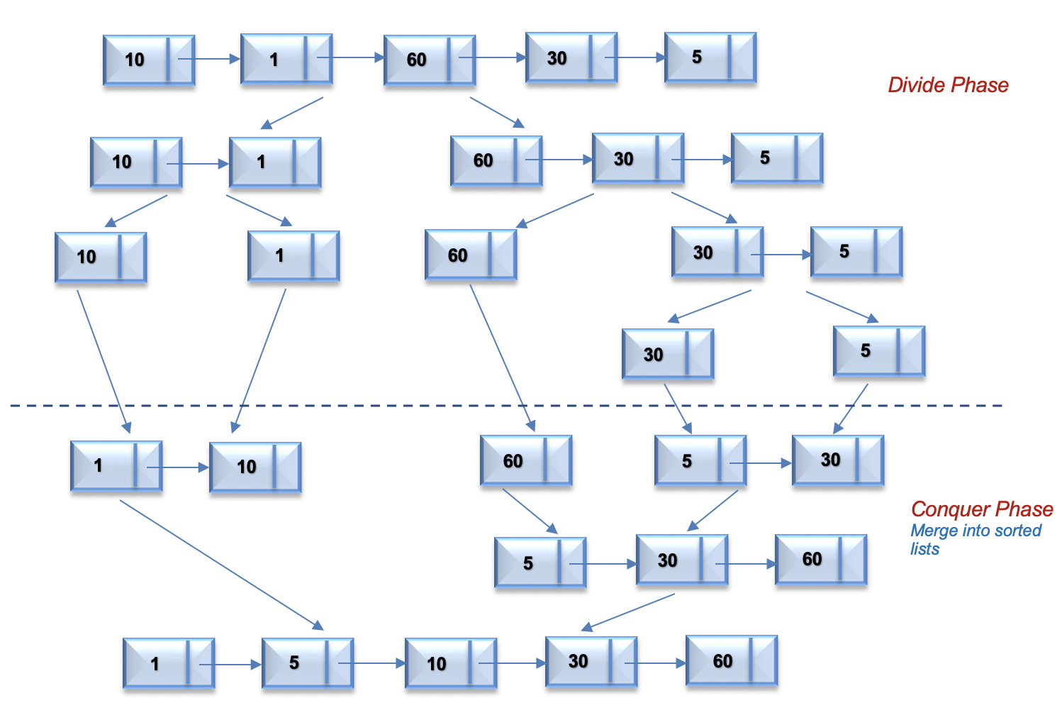
- Divide phase: Recursively split the original list into two halves. The split continues until there is only one node in the linked list. To split the list into two halves, we find the middle of the linked list using the Fast and Slow pointer approach as mentioned in Find Middle Of Linked List.
- Merge phase: Recursively sort each sublist and combine it into a single sorted list. (Merge Phase). This is similar to the problem Merge two sorted linked lists
- The process continues until we get the original list in sorted order.
- For the linked list =
[10,1,60,30,5], the following figure illustrates the merge sort process using a top down approach.
- The algorithm is as follows:
- Let the head be the first node of the linked list to be sorted and
headRefbe the pointer to head. Note that we need a reference to head inMergeSort()as the below implementation changes next links to sort the linked lists (not data at the nodes), so the head node has to be changed if the data at the original head is not the smallest value in the linked list.
MergeSort(headRef)
1) If the head is NULL or there is only one element in the Linked List
    then return.
2) Else divide the linked list into two halves.
      FrontBackSplit(head, &a, &b); /* a and b are two halves */
3) Sort the two halves a and b.
      MergeSort(a);
      MergeSort(b);
4) Merge the sorted a and b (using SortedMerge())
   and update the head pointer using headRef.
     *headRef = SortedMerge(a, b);
# Python3 program to merge sort of linked list

# create Node using class Node.
class Node:
    def __init__(self, data):
        self.data = data
        self.next = None

class LinkedList:
    def __init__(self):
        self.head = None

    # push new value to linked list
    # using append method
    def append(self, new_value):

        # Allocate new node
        new_node = Node(new_value)

        # if head is None, initialize it to new node
        if not self.head:
            self.head = new_node
            return
        curr_node = self.head
        while curr_node.next:
            curr_node = curr_node.next

        # Append the new node at the end
        # of the linked list
        curr_node.next = new_node

    def sortedMerge(self, a, b):
        result = None

        # Base cases
        if not a:
            return b
        if not b:
            return a

        # pick either a or b and recur..
        if a.data <= b.data:
            result = a
            result.next = self.sortedMerge(a.next, b)
        else:
            result = b
            result.next = self.sortedMerge(a, b.next)
        return result

    def mergeSort(self, head):
        # Base case if head is None
        if not head or not head.next:
            return head

        # get the middle of the list
        middle = self.getMiddle(h)
        middleNext = middle.next

        # set the next of middle node to None
        middle.next = None

        # Apply mergeSort on left list
        left = self.mergeSort(head)

        # Apply mergeSort on right list
        right = self.mergeSort(middleNext)

        # Merge the left and right lists
        sortedList = self.sortedMerge(left, right)
        return sortedList

    # Utility function to get the middle
    # of the linked list
    # using The Tortoise and The Hare approach
    def getMiddle(self, head):
        if not head:
            return head

        slow = head
        fast = head

        while fast.next and fast.next.next:
            slow = slow.next
            fast = fast.next.next

        return slow

# Utility function to print the linked list
def printList(head):
    if head is None:
        print(' ')
        return

    curr_node = head
    while curr_node:
        print(curr_node.data, end = " ")
        curr_node = curr_node.next

    print(' ')

# Driver Code
if __name__ == '__main__':
    li = LinkedList()

    # Let us create a unsorted linked list
    # to test the functions created.
    # The list shall be a: 2->3->20->5->10->15
    li.append(15)
    li.append(10)
    li.append(5)
    li.append(20)
    li.append(3)
    li.append(2)

    # Apply merge Sort
    li.head = li.mergeSort(li.head)
    print ("Sorted Linked List is:")
    printList(li.head)
- which outputs:
Sorted Linked List is:
2 3 5 10 15 20
Complexity
- Time: \(O(n\log{n})\) (both average and worst-case performance), where \(n\) is the number of nodes in linked list. The algorithm can be split into two phases, split and merge.
- Let’s assume that \(n\) is power of 2. For n = 16, the split and merge operation in Top Down fashion can be visualized as follows:

- Split:
- The recursion tree expands in form of a complete binary tree, splitting the list into two halves recursively. The number of levels in a complete binary tree is given by \(\log_{2} n\). For \(n=16\), number of splits = \(\log_{2} 16 = 4\).
- Merge:
- At each level, we merge \(n\) nodes which takes \(\mathcal{O}(n)\) time. For \(n = 16\), we perform merge operation on 16 nodes in each of the 44 levels.
- So the time complexity for split and merge operation is \(\mathcal{O}(n \log n)\).
- Split:
- Let’s assume that \(n\) is power of 2. For n = 16, the split and merge operation in Top Down fashion can be visualized as follows:
- Space: \(O(n\log{n})\), where \(n\) is the number of nodes in linked list. Since the problem is recursive, we need additional space to store the recursive call stack. The maximum depth of the
mergeSort()recursion tree is \(\log n\) and the maximum depth of thesortedMerge()recursion tree is \(n\).
Solution: Bottom Up/Iterative Merge Sort (better space complexity); recursively split the list into two parts, merge the two resulting sorted lists
- Intuition:
- The Top Down Approach for merge sort uses \(\mathcal{O}(\log n)\) extra space due to recursive call stack. Let’s understand how we can implement merge sort using constant extra space using Bottom Up Approach.
- The Bottom Up approach for merge sort starts by splitting the problem into the smallest subproblem and iteratively merge the result to solve the original problem.
- First, the list is split into sublists of size 1 and merged iteratively in sorted order. The merged list is solved similarly.
- The process continues until we sort the entire list.
- This approach is solved iteratively and can be implemented using constant extra space. Let’s look at the algorithm to implement merge sort in Bottom Up Fashion.
- Algorithm:
mergeSort():- If the size of the linked list is 1 then return the
head. - Find
midusing The Tortoise and The Hare Approach - Store the next of
midinb, i.e., the right sub-linked list. - Now make the next midpoint
None. - Recursively call
mergeSort()on both left and right sub-linked list and store the new head of the left and right linked list. - Call
sortedMerge()given the arguments new heads of left and right sub-linked lists and store the final head returned after merging. - Return the final head of the merged linkedlist.
- If the size of the linked list is 1 then return the
merge(a, b):- Create a dummy node with fake data (say
-1), sayresult, to store the merged list after sorting in itsnextand store a dummy node in it. - Take a pointer
tempand assignmergeto it. - If the data of
ais less than the data ofb, then, storeain next of temp and moveato the next ofa. - Else store
bin next of temp and movebto the next ofb. - Move
tempto the next oftemp. - Repeat steps 3, 4 and 5 until
ais not equal toNoneandbis not equal toNone. - Now add any remaining nodes of the first or the second linked list to the merged linked list.
- Return the
nextofresult(that will ignore the dummy node and return the head of the final merged linked list)
- Create a dummy node with fake data (say
- For the linked
list = [10,1,30,2,5], the following figure illustrates the merge sort process using a Bottom Up approach.
# Node Class
class Node:
    def __init__(self, key):
        self.data = key
        self.next = None

class LinkedList:
    def __init__(self):
        self.head = None

    # Function to merge sort
    def mergeSort(self, head: Optional[ListNode]) -> Optional[ListNode]:
        # Base case if head is None
        if not head or not head.next:
            return head

        # get the middle of the list
        middle = self.getMiddle(head)
        middleNext = middle.next

        # set the next of middle node to None
        middle.next = None

        # Apply mergeSort on left list
        left = self.mergeSort(head)

        # Apply mergeSort on right list
        right = self.mergeSort(middleNext)

        # Merge the left and right lists
        sortedList = self.sortedMerge(left, right)
        return sortedList

    # Function to merge two linked lists
    def sortedMerge(self, a, b):
        # Base cases
        if not a:
            return b
        if not b:
            return a

        # dummy node
        result = Node(-1)
        temp = result

        # while a is not null and b
        # is not None
        while a and b:
            if a.data < b.data:
                temp.next = a
                a = a.next
            else:
                temp.next = b
                b = b.next
            temp = temp.next

        # while a is not null
        while a:
            temp.next = a
            a = a.next
            temp = temp.next

        # while b is not null
        while b:
            temp.next = b
            b = b.next
            temp = temp.next

        return result.next

    # Utility function to get the middle
    # of the linked list
    # using The Tortoise and The Hare approach
    def getMiddle(self, head):
        if not head:
            return head

        slow = head
        fast = head

        while fast.next and fast.next.next:
            slow = slow.next
            fast = fast.next.next

        return slow

    # Function to print list
    def printList(head):
        while head:
            print(head.data, end=" ")
            head = head.next

# Driver Code
head = Node(7)
temp = head
temp.next = Node(10);
temp = temp.next;
temp.next = Node(5);
temp = temp.next;
temp.next = Node(20);
temp = temp.next;
temp.next = Node(3);
temp = temp.next;
temp.next = Node(2);
temp = temp.next;

# Apply merge Sort
head = mergeSort(head);
print("\nSorted Linked List is: \n");

printList(head)
- which outputs:
Sorted Linked List is:
2 3 5 7 10 20
Complexity
- Time: \(O(n\log{n})\) (both average and worst-case performance), where \(n\) is the number of nodes in linked list. Let’s analyze the time complexity of each step:
- Count Nodes: Get the count of number nodes in the linked list requires \(\mathcal{O}(n)\) time.
- Split and Merge: This operation is similar to Approach 1 and takes \(\mathcal{O}(n \log n)\) time. For \(n = 16\), the split and merge operation in Bottom Up fashion can be visualized as follows

- This gives us total time complexity as \(\mathcal{O}(n)\) + \(\mathcal{O}(n \log n)\) = \(\mathcal{O}(n \log n)\).
- Space: O(\log{n})$$ for
mergSort()recursion. Also, note that storing the reference pointerstail,nextSubListetc. only uses constant space.
Further Reading
[912/Medium] Sort an Array
Problem
-
Given an array of integers
nums, sort the array in ascending order. -
Example 1:
Input: nums = [5,2,3,1]
Output: [1,2,3,5]
- Example 2:
Input: nums = [5,1,1,2,0,0]
Output: [0,0,1,1,2,5]
- Constraints:
1 <= nums.length <= 5 * 104-5 * 104 <= nums[i] <= 5 * 104
-
Follow up: Can you sort the linked list in
O(n logn)time andO(1)memory (i.e. constant space)? - See problem on LeetCode.
Solution: QuickSort
- Algorithm:
- Like Merge Sort, QuickSort is a Divide and Conquer algorithm. It picks an element as pivot and partitions the given array around the picked pivot. There are many different versions of quickSort that pick pivot in different ways.
- Always pick first element as pivot.
- Always pick last element as pivot (implemented below)
- Pick a random element as pivot.
- Pick median as pivot.
- The key process in quickSort is
partition(). Target of partitions is, given an array and an elementxof array as pivot, putxat its correct position in sorted array and put all smaller elements (smaller thanx) beforex, and put all greater elements (greater thanx) afterx. All this should be done in linear time.
- Like Merge Sort, QuickSort is a Divide and Conquer algorithm. It picks an element as pivot and partitions the given array around the picked pivot. There are many different versions of quickSort that pick pivot in different ways.
Recursive QuickSort
- Pseudo Code for recursive QuickSort function:
/* low  --> Starting index,  high  --> Ending index */
quickSort(arr[], low, high)
{
    if (low < high)
    {
        /* pi is partitioning index, arr[pi] is now
           at right place */
        pi = partition(arr, low, high);

        quickSort(arr, low, pi - 1);  // Before pi
        quickSort(arr, pi + 1, high); // After pi
    }
}

Partition Algorithm
- There can be many ways to do partition, following pseudo code adopts the method given in CLRS book. The logic is simple, we start from the leftmost element and keep track of index of smaller (or equal to) elements as
i. While traversing, if we find a smaller element, we swap current element witharr[i]. Otherwise we ignore current element.
/* low  --> Starting index,  high  --> Ending index */
quickSort(arr[], low, high)
{
    if (low < high)
    {
        /* pi is partitioning index, arr[pi] is now
           at right place */
        pi = partition(arr, low, high);

        quickSort(arr, low, pi - 1);  // Before pi
        quickSort(arr, pi + 1, high); // After pi
    }
}
Pseudo code for partition()
/* This function takes last element as pivot, places
   the pivot element at its correct position in sorted
    array, and places all smaller (smaller than pivot)
   to left of pivot and all greater elements to right
   of pivot */
partition (arr[], low, high)
{
    // pivot (Element to be placed at right position)
    pivot = arr[high];

    i = (low - 1)  // Index of smaller element and indicates the
                   // right position of pivot found so far

    for (j = low; j <= high- 1; j++)
    {
        // If current element is smaller than the pivot
        if (arr[j] < pivot)
        {
            i++;    // increment index of smaller element
            swap arr[i] and arr[j]
        }
    }
    swap arr[i + 1] and arr[high])
    return (i + 1)
}
Illustration of partition()
arr[] = {10, 80, 30, 90, 40, 50, 70}
Indexes:  0   1   2   3   4   5   6

low = 0, high =  6, pivot = arr[h] = 70
Initialize index of smaller element, i = -1

Traverse elements from j = low to high-1
j = 0 : Since arr[j] <= pivot, do i++ and swap(arr[i], arr[j])
i = 0
arr[] = {10, 80, 30, 90, 40, 50, 70} // No change as i and j
                                     // are same

j = 1 : Since arr[j] > pivot, do nothing
// No change in i and arr[]

j = 2 : Since arr[j] <= pivot, do i++ and swap(arr[i], arr[j])
i = 1
arr[] = {10, 30, 80, 90, 40, 50, 70} // We swap 80 and 30

j = 3 : Since arr[j] > pivot, do nothing
// No change in i and arr[]

j = 4 : Since arr[j] <= pivot, do i++ and swap(arr[i], arr[j])
i = 2
arr[] = {10, 30, 40, 90, 80, 50, 70} // 80 and 40 Swapped
j = 5 : Since arr[j] <= pivot, do i++ and swap arr[i] with arr[j]
i = 3
arr[] = {10, 30, 40, 50, 80, 90, 70} // 90 and 50 Swapped

We come out of loop because j is now equal to high-1.
Finally we place pivot at correct position by swapping
arr[i+1] and arr[high] (or pivot)
arr[] = {10, 30, 40, 50, 70, 90, 80} // 80 and 70 Swapped

Now 70 is at its correct place. All elements smaller than
70 are before it and all elements greater than 70 are after
it.
- Why Quick Sort is preferred over MergeSort for sorting Arrays:
- Quick Sort in its general form is an in-place sort (i.e., it doesn’t require any extra storage) whereas merge sort requires \(O(n)\) extra storage, \(n\) denoting the array size which may be quite expensive. Allocating and de-allocating the extra space used for merge sort increases the running time of the algorithm. Comparing average complexity we find that both type of sorts have \(O(n\log{n})\) average complexity but the constants differ. For arrays, merge sort loses due to the use of extra \(O(n)\) storage space.
- Most practical implementations of Quick Sort use randomized version. The randomized version has expected time complexity of \(O(nLogn)\). The worst case is possible in randomized version also, but worst case doesn’t occur for a particular pattern (like sorted array) and randomized Quick Sort works well in practice.
- Quick Sort is also a cache friendly sorting algorithm as it has good locality of reference when used for arrays.
- Quick Sort is also tail recursive, therefore tail call optimizations is done.
- Why MergeSort is preferred over QuickSort for Linked Lists?:
- In case of linked lists the case is different mainly due to difference in memory allocation of arrays and linked lists. Unlike arrays, linked list nodes may not be adjacent in memory. Unlike array, in linked list, we can insert items in the middle in \(O(1)\) extra space and \(O(1)\) time. Therefore merge operation of merge sort can be implemented without extra space for linked lists.
- In arrays, we can do random access as elements are continuous in memory. Let us say we have an integer (4-byte) array \(A\) and let the address of
A[0]bexthen to accessA[i], we can directly access the memory at (\(x + i*4\)). Unlike arrays, we can not do random access in linked list. Quick Sort requires a lot of this kind of access. In linked list to access \(i^{th}\) index, we have to travel each and every node from the head to \(i^{th}\) node as we don’t have continuous block of memory. Therefore, the overhead increases for quick sort. Merge sort accesses data sequentially and the need of random access is low.
class SortArray:
    def sortArray(self, nums: List[int]) -> List[int]:
        self.quicksort(nums, 0, len(nums)-1)
        return nums

    # Function to perform quicksort
    def quick_sort(self, nums, low, high):
        if low < high:
            # Find pivot element such that
            # element smaller than pivot are on the left
            # element greater than pivot are on the right
            pi = self.partition(nums, low, high)

            # Recursive call on the left of pivot
            self.quick_sort(nums, low, pi - 1)

            # Recursive call on the right of pivot
            self.quick_sort(nums, pi + 1, high)

    # Function to find the partition position
    def partition(self, nums, low, high):

        # Choose the rightmost element as pivot
        pivot = nums[high]

        # Pointer for greater element
        i = low - 1

        # Traverse through all elements
        # compare each element with pivot
        for j in range(low, high):
            if nums[j] <= pivot:
                # If element smaller than pivot is found
                # swap it with the greater element pointed by i
                i += 1

                # Swapping element at i with element at j
                nums[i], nums[j] = nums[j], nums[i]

        # Swap the pivot element with the greater element specified by i
        nums[i + 1], nums[high] = nums[high], nums[i + 1]

        # Return the position from where partition is done
        return i + 1

# Driver code
nums = [10, 7, 8, 9, 1, 5]
SortArray().sortArray(nums)
# or SortArray().quick_sort(nums, 0, len(nums) - 1)

print(f'Sorted array: {nums}')
- which outputs:
Sorted array:
1 5 7 8 9 10
Complexity
- Time: \(O(n\log{n})\) (average performance) and \(O(n^2)\) (worst-case performance), where \(n\) is the number of nodes in linked list.
- Space: \(O(\log{n})\) (average performance) and \(O(n)\) (worst-case performance).
- The worst case arises when the sort is not balanced. However it can be avoided by sorting the smaller sub-arrays first and then tail-recursing on the larger array. This improved version will have a worst case space complexity of \(O(\log{n})\). Note that the tail recursion is internally implemented by most compilers and no extra code needs to be written for that.
- Merge sort has an average/worst case space complexity of \(O(n)\) because the merge subroutine copies the array to a new array which requires \(O(n)\) extra space.
When does the worst case of Quicksort occur?
- The worst case time complexity of a typical implementation of QuickSort is \(O(n^2)\) which can be hit depending on the strategy for choosing pivot. In early versions of Quick Sort, where the picked pivot is always an extreme (smallest or largest) element, i.e., the leftmost (or rightmost) element is chosen as a pivot, the worst occurs in the following cases.
- Array is already sorted in the same order.
- Array is already sorted in reverse order.
- All elements are the same (a special case of cases 1 and 2)
- Thus, the worst case of Quicksort happens when input array is sorted or reverse sorted and either first or last element is picked as pivot.
- Since these cases are very common to use cases, the problem can easily be solved by choosing either a random index for the pivot, choosing the middle index of the partition, or (especially for longer partitions) choosing the median of the first, middle and last element of the partition for the pivot. With these modifications, the worst case of Quicksort has fewer chances to occur, but a worst case can still occur if the input array is such that the maximum (or minimum) element is always chosen as the pivot.
- Although randomized QuickSort works well even when the array is sorted, there is still possible that the randomly picked element is always extreme.