Distilled • LeetCode • Grid

• Pattern: Grid
  • [73/Medium] Set Matrix Zeroes
    • Problem
    • Solution: Book-keep rows and cols to be set to 0
    • Complexity
    • Solution: treat first cell of every row and column as a flag
      • Complexity
  • [79/Medium] Word Search
    • Problem
    • Solution: Backtracking
    • Complexity
  • [130/Medium] Surrounded Regions
    • Problem
    • Solution: DFS
      • Complexity
    • Solution: BFS
      • Complexity
  • [361/Medium] Bomb Enemy
    • Problem
    • Solution: Brute-force
      • Complexity
    • Solution: Dynamic Programming
      • Complexity
  • [733/Easy] Flood Fill
    • Problem
    • Solution: DFS
      • Complexity
  • [827/Hard] Making A Large Island
    • Problem
    • Solution: Naive DFS
      • Complexity
    • Solution: Backtracking/DFS
      • Complexity
    • Solution: Component Sizes
      • Complexity
  • [994/Medium] Rotting Oranges
    • Problem
    • Solution: BFS
      • Complexity
    • Solution: BFS with counter for fresh
      • Complexity
    • Solution: In-place BFS
      • Complexity
  • [1091/Medium] Shortest Path in Binary Matrix
    • Problem
    • Solution: BFS
    • Solution: BFS + Deque
    • Solution: A* search
      • Concept
  • [1275/Easy] Find Winner on a Tic Tac Toe Game
    • Problem
    • Solution: Alternate between players, check for the four wining conditions
      • Complexity
    • Solution: Record Each Move
      • Complexity
  • [1293/Hard] Shortest Path in a Grid with Obstacles Elimination
    • Problem
    • Solution: Trivial BFS
      • Complexity
    • Solution: Enhanced BFS
    • Solution: Nuanced BFS

Pattern: Grid

[73/Medium] Set Matrix Zeroes

Problem

• Given an m x n integer matrix matrix, if an element is 0, set its entire row and column to 0’s.

• You must do it in place.

• Example 1:

Input: matrix = [[1,1,1],[1,0,1],[1,1,1]]
Output: [[1,0,1],[0,0,0],[1,0,1]]

• Example 2:

Input: matrix = [[0,1,2,0],[3,4,5,2],[1,3,1,5]]
Output: [[0,0,0,0],[0,4,5,0],[0,3,1,0]]

• Constraints:
  • m == matrix.length
  • n == matrix[0].length
  • 1 <= m, n <= 200
  • -231 <= matrix[i][j] <= 231 - 1
• Follow up:
  • A straightforward solution using \(O(mn)\) space is probably a bad idea.
  • A simple improvement uses \(O(m + n)\) space, but still not the best solution.
  • Could you devise a constant space solution?

Solution: Book-keep rows and cols to be set to 0

• Intuition:
  • If any cell of the matrix has a zero we can record its row and column number. All the cells of this recorded row and column can be marked zero in the next iteration.
• Algorithm:
  • We make a pass over our original array and look for zero entries.
  • If we find that an entry at [i, j] is 0, then we need to record somewhere the row i and column j.
  • So, we use two sets, one for the rows and one for the columns.

      if cell[i][j] == 0 {
      row_set.add(i)
      column_set.add(j)
      }
    

  • Finally, we iterate over the original matrix. For every cell we check if the row r or column c had been marked earlier. If any of them was marked, we set the value in the cell to 0.

      if r in row_set or c in column_set {
      cell[r][c] = 0
      }
    

class Solution(object):
    def setZeroes(self, matrix):
        """
        :type matrix: List[List[int]]
        :rtype: void Do not return anything, modify matrix in-place instead.
        """
        R = len(matrix)
        C = len(matrix[0])
        rows, cols = set(), set()

        # Essentially, we mark the rows and columns that are to be made zero
        for i in range(R):
            for j in range(C):
                if matrix[i][j] == 0:
                    rows.add(i)
                    cols.add(j)

        # Iterate over the array once again and using the rows and cols sets, update the elements
        for i in range(R):
            for j in range(C):
                if i in rows or j in cols:
                    matrix[i][j] = 0                

Complexity

• Time: \(O(mn)\) where \(m\) and \(n\) are the number of rows and columns respectively.
• Space: \(O(m+n)\)

Solution: treat first cell of every row and column as a flag

• Intuition:
  • Rather than using additional variables to keep track of rows and columns to be reset, we use the matrix itself as the indicators.

    The idea is that we can use the first cell of every row and column as a flag. This flag would determine whether a row or column has been set to zero. This means for every cell instead of going to \(M+N\) cells and setting it to zero we just set the flag in two cells.

      if cell[i][j] == 0 {
      cell[i][0] = 0
      cell[0][j] = 0
      }
    

  • These flags are used later to update the matrix. If the first cell of a row is set to zero this means the row should be marked zero. If the first cell of a column is set to zero this means the column should be marked zero.
• Algorithm:
  • We iterate over the matrix and we mark the first cell of a row i and first cell of a column j, if the condition in the pseudo code above is satisfied. i.e., if cell[i][j] == 0.
  • The first cell of row and column for the first row and first column is the same, i.e., cell[0][0]. Hence, we use an additional variable to tell us if the first column had been marked or not and the cell[0][0] would be used to tell the same for the first row.
  • Now, we iterate over the original matrix starting from second row and second column, i.e., matrix[1][1] onwards. For every cell we check if the row r or column c had been marked earlier by checking the respective first row cell or first column cell. If any of them was marked, we set the value in the cell to 0. Note the first row and first column serve as the row_set and column_set that we used in the first approach.
  • We then check if cell[0][0] == 0, if this is the case, we mark the first row as zero.
  • And finally, we check if the first column was marked, we make all entries in it as zeros.
• In the above animation we iterate all the cells and mark the corresponding first row/column cell incase of a cell with zero value.

• We iterate the matrix we got from the above steps and mark respective cells zeroes.

class Solution(object):
    def setZeroes(self, matrix):
        """
        :type matrix: List[List[int]]
        :rtype: void Do not return anything, modify matrix in-place instead.
        """
        is_col = False
        R = len(matrix)
        C = len(matrix[0])
        for i in range(R):
            # Since first cell for both first row and first column is the same i.e. matrix[0][0]
            # We can use an additional variable for either the first row/column.
            # For this solution we are using an additional variable for the first column
            # and using matrix[0][0] for the first row.
            if matrix[i][0] == 0:
                is_col = True
            for j in range(1, C):
                # If an element is zero, we set the first element of the corresponding row and column to 0
                if matrix[i][j]  == 0:
                    matrix[0][j] = 0
                    matrix[i][0] = 0

        # Iterate over the array once again and using the first row and first column, update the elements.
        for i in range(1, R):
            for j in range(1, C):
                if not matrix[i][0] or not matrix[0][j]:
                    matrix[i][j] = 0

        # See if the first row needs to be set to zero as well
        if matrix[0][0] == 0:
            for j in range(C):
                matrix[0][j] = 0

        # See if the first column needs to be set to zero as well        
        if is_col:
            for i in range(R):
                matrix[i][0] = 0

Complexity

• Time: \(O(m \times n)\)
• Space: \(O(1)\)

[79/Medium] Word Search

Problem

• Given an m x n grid of characters board and a string word, return true if word exists in the grid.

• The word can be constructed from letters of sequentially adjacent cells, where adjacent cells are horizontally or vertically neighboring. The same letter cell may not be used more than once.

• Example 1:

Input: board = [["A","B","C","E"],["S","F","C","S"],["A","D","E","E"]], word = "ABCCED"
Output: true

• Example 2:

Input: board = [["A","B","C","E"],["S","F","C","S"],["A","D","E","E"]], word = "SEE"
Output: true

• Example 3:

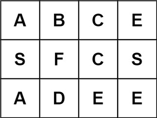
Input: board = [["A","B","C","E"],["S","F","C","S"],["A","D","E","E"]], word = "ABCB"
Output: false

• Constraints:
  • m == board.length
  • n = board[i].length
  • 1 <= m, n <= 6
  • 1 <= word.length <= 15
  • board and word consists of only lowercase and uppercase English letters.

Follow up: Could you use search pruning to make your solution faster with a larger board?

• See problem on LeetCode.

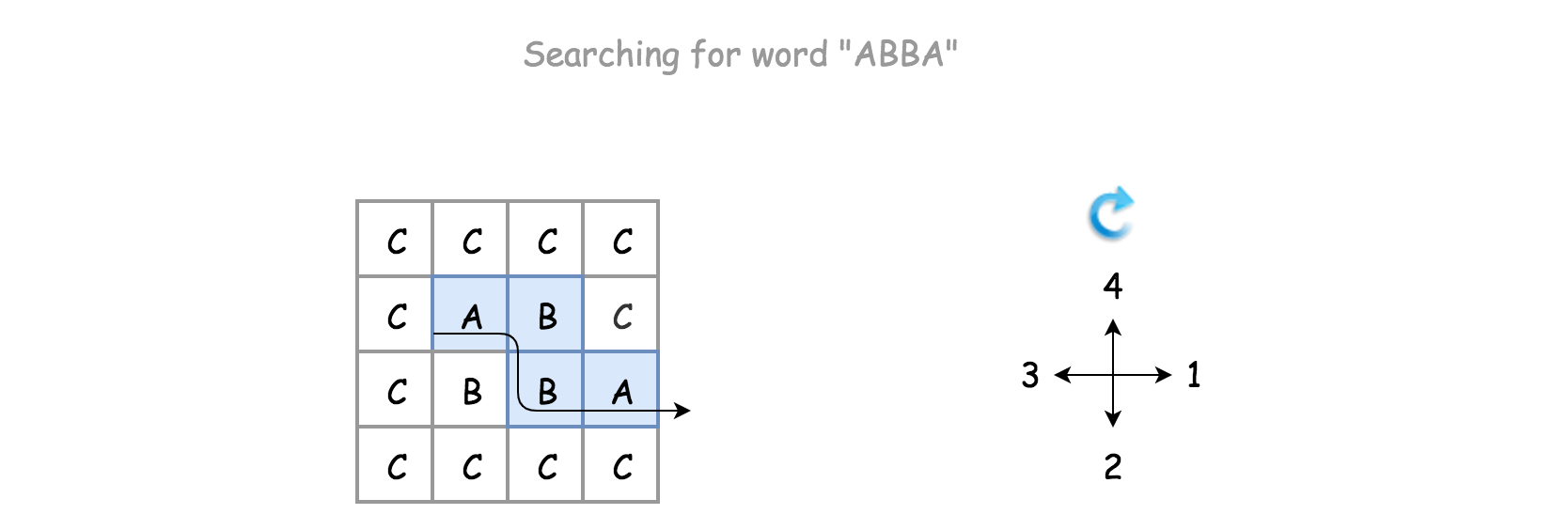
Solution: Backtracking

• Intuition:
  • This problem is yet another 2D grid traversal problem, which is similar with another problem called 489. Robot Room Cleaner.
  • Many people in the discussion forum claimed that the solution is of DFS (Depth-First Search). Although it is true that we would explore the 2D grid with the DFS strategy for this problem, it does not capture the entire nature of the solution.
  • We argue that a more accurate term to summarize the solution would be backtracking, which is a methodology where we mark the current path of exploration, if the path does not lead to a solution, we then revert the change (i.e. backtracking) and try another path.
  • As the general idea for the solution, we would walk around the 2D grid, at each step we mark our choice before jumping into the next step. And at the end of each step, we would also revert our marking, so that we could have a clean slate to try another direction. In addition, the exploration is done via the DFS strategy, where we go as further as possible before we try the next direction.

  

• Algorithm:
  • There is a certain code pattern for all the algorithms of backtracking.
  • The skeleton of the algorithm is a loop that iterates through each cell in the grid. For each cell, we invoke the backtracking function (i.e. backtrack()) to check if we would obtain a solution, starting from this very cell.
  • For the backtracking function backtrack(row, col, suffix), as a DFS algorithm, it is often implemented as a recursive function. The function can be broke down into the following four steps:
  • Step 1). At the beginning, first we check if we reach the bottom case of the recursion, where the word to be matched is empty, i.e. we have already found the match for each prefix of the word.
  • Step 2). We then check if the current state is invalid, either the position of the cell is out of the boundary of the board or the letter in the current cell does not match with the first letter of the current suffix.
  • Step 3). If the current step is valid, we then start the exploration of backtracking with the strategy of DFS. First, we mark the current cell as visited, e.g. any non-alphabetic letter will do. Then we iterate through the four possible - directions, namely up, right, down and left. The order of the directions can be altered, to one’s preference.
  • Step 4). At the end of the exploration, we revert the cell back to its original state. Finally, we return the result of the exploration.

• Note that instead of returning directly once we find a match (in backtrack()), we simply break out of the loop and do the cleanup before returning. In other words, we simply return True if the result of recursive call to backtrack() is positive. Though this minor modification would have no impact on the time or space complexity, it would however leave with some “side-effect”, i.e. the matched letters in the original board would be altered to #.

• Instead of doing the boundary checks before the recursive call on the backtrack() function, we do it within the function. This is an important choice though. Doing the boundary check within the function would allow us to reach the base case, for the test case where the board contains only a single cell, since either of neighbor indices would not be valid.

class Solution(object):
    def exist(self, board, word):
        """
        :type board: List[List[str]]
        :type word: str
        :rtype: bool
        """
        self.rows = len(board)
        self.cols = len(board[0])
        self.board = board

        # iterate through each character on the board
        for row in range(self.rows):
            for col in range(self.cols):
                if self.backtrack(row, col, word):
                    return True

        # no match found after all exploration
        return False


    def backtrack(self, row, col, suffix):
        # base case: we find match for each letter in the word
        if len(suffix) == 0:
            return True

        # Check the current status, before jumping into backtracking
        if row < 0 or row == self.rows or col < 0 or col == self.cols \
                #next character is not subsequent
                or self.board[row][col] != suffix[0]:
            return False

        ret = False
        # mark the choice before exploring further.
        self.board[row][col] = '#'
        # explore the 4 neighbor/adjacent directions
        for rowOffset, colOffset in [(0, 1), (1, 0), (0, -1), (-1, 0)]:
            # ret = self.backtrack(row + rowOffset, col + colOffset, suffix[1:])
            # break instead of return directly to do some cleanup afterwards
            # if ret: break
            
            # sudden-death return, no cleanup.
            if self.backtrack(row + rowOffset, col + colOffset, suffix[1:]):
                return True            

        # revert the change, a clean slate and no side-effect
        self.board[row][col] = suffix[0]

        # Tried all directions, and did not find any match
        return ret

Complexity

• Time: \(O(m*n*3^len(word)) (or\)O(n*3^l)\(), where\)O(DFS Traversal)\(=\)3^len(word)\(,\)n\(is the number of cells in the board and\)l$$ is the length of the word to be matched.
  • For the backtracking function, initially we could have at most 4 directions to explore, but further the choices are reduced into 3 (since we won’t go back to where we come from). As a result, the execution trace after the first step could be visualized as a 3-ary tree, each of the branches represent a potential exploration in the corresponding direction. Therefore, in the worst case, the total number of invocation would be the number of nodes in a full 3-nary tree, which is about \(3^L\).
  • We iterate through the board for backtracking, i.e., there could be \(n\) times invocation for the backtracking function in the worst case.
  • As a result, overall the time complexity of the algorithm would be \(O(n*3^l)\)
• Space: \(O(len(word))\) or \(O(l)\) where \(l\) is the length of the word to be matched. The main consumption of the memory lies in the recursion callstack of the backtracking function. The maximum length of the call stack would be the length of the word. Therefore, the space complexity of the algorithm is \(O(l)\).

[130/Medium] Surrounded Regions

Problem

• Given an m x n matrix board containing 'X' and 'O', capture all regions that are 4-directionally surrounded by 'X'.

• A region is captured by flipping all ‘O’s into ‘X’s in that surrounded region.

• Example 1:

Input: board = [["X","X","X","X"],["X","O","O","X"],["X","X","O","X"],["X","O","X","X"]]
Output: [["X","X","X","X"],["X","X","X","X"],["X","X","X","X"],["X","O","X","X"]]
Explanation: Surrounded regions should not be on the border, which means that any 'O' on the border of the board are not flipped to 'X'. Any 'O' that is not on the border and it is not connected to an 'O' on the border will be flipped to 'X'. Two cells are connected if they are adjacent cells connected horizontally or vertically.

• Example 2:

Input: board = [["X"]]
Output: [["X"]]

• Constraints:
  • m == board.length
  • n == board[i].length
  • 1 <= m, n <= 200
  • board[i][j] is 'X' or 'O'.
• See problem on LeetCode.

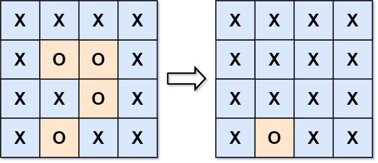
Solution: DFS

• Overview:
  • This problem is almost identical as the capture rule of the Go game, where one captures the opponent’s stones by surrounding them. The difference is that in the Go game the borders of the board are considered to the walls that surround the stones, while in this problem a group of cells (i.e. region) is considered to be escaped from the surrounding if it reaches any border.

  

  • This problem is yet another problem concerning the traversal of 2D grid, e.g. Robot Room Cleaner.

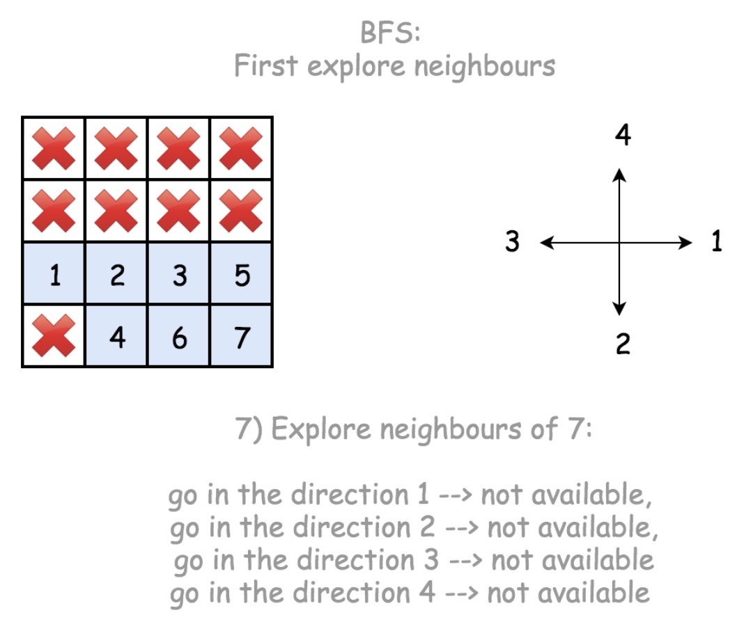
  As similar to the traversal problems in a tree structure, there are generally two approaches in terms of solution: DFS (Depth-First Search) and BFS (Breadth-First Search).

  • One can apply either of the above strategies to traverse the 2D grid, while taking some specific actions to resolve the problems.

  • Given a traversal strategy (DFS or BFS), there could be a thousand implementations for a thousand people, if we indulge ourselves to exaggerate a bit. However, there are some common neat techniques that we could apply along with both of the strategies, in order to obtain a more optimized solution.

• Intuition:

  The goal of this problem is to mark those captured cells.

  • If we are asked to summarize the algorithm in one sentence, it would be that we enumerate all those candidate cells (i.e. the ones filled with O), and check one by one if they are captured or not, i.e. we start with a candidate cell (O), and then apply either DFS or BFS strategy to explore its surrounding cells.
• Algorithm:
  • Let us start with the DFS algorithm, which usually results in a more concise code than the BFS algorithm. The algorithm consists of three steps:
    • Step 1). We select all the cells that are located on the borders of the board.
    • Step 2). Start from each of the above selected cell, we then perform the DFS traversal.
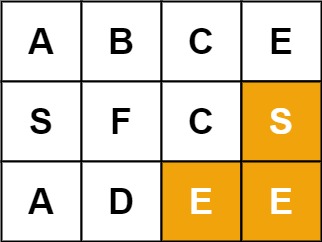
      • If a cell on the border happens to be O, then we know that this cell is alive, together with the other O cells that are connected to this border cell, based on the description of the problem. Two cells are connected, if there exists a path consisting of only O letter that bridges between the two cells.
      • Based on the above conclusion, the goal of our DFS traversal would be to mark out all those connected O cells that is originated from the border, with any distinguished letter such as E.
  • Step 3). Once we iterate through all border cells, we would then obtain three types of cells:
    • The one with the X letter: the cell that we could consider as the wall.
    • The one with the O letter: the cells that are spared in our DFS traversal, i.e. these cells has no connection to the border, therefore they are captured. We then should replace these cell with X letter.
  • The one with the E letter: these are the cells that are marked during our DFS traversal, i.e. these are the cells that has at least one connection to the borders, therefore they are not captured. As a result, we would revert the cell to its original letter O.
  • We demonstrate how the DFS works with an example in the following animation.

class Solution(object):
    def solve(self, board):
        """
        :type board: List[List[str]]
        :rtype: None Do not return anything, modify board in-place instead.
        """
        if not board or not board[0]:
            return

        self.ROWS = len(board)
        self.COLS = len(board[0])

        # Step 1). retrieve all border cells
        from itertools import product
        borders = list(product(range(self.ROWS), [0, self.COLS-1])) \
                + list(product([0, self.ROWS-1], range(self.COLS)))

        # Step 2). mark the "escaped" cells, with any placeholder, e.g. 'E'
        for row, col in borders:
            self.DFS(board, row, col)

        # Step 3). flip the captured cells ('O'->'X') and the escaped one ('E'->'O')
        for r in range(self.ROWS):
            for c in range(self.COLS):
                if board[r][c] == 'O':   board[r][c] = 'X'  # captured
                elif board[r][c] == 'E': board[r][c] = 'O'  # escaped


    def DFS(self, board, row, col):
        if board[row][col] != 'O':
            return
            
        board[row][col] = 'E'
        
        if col < self.COLS-1: 
            self.DFS(board, row, col+1)
        
        if row < self.ROWS-1: 
            self.DFS(board, row+1, col)
        
        if col > 0: 
            self.DFS(board, row, col-1)
        
        if row > 0: 
            self.DFS(board, row-1, col)

• Optimizations:
  • In the above implementation, there are a few techniques that we applied under the hood, in order to further optimize our solution. Here we list them one by one.

    Rather than iterating all candidate cells (the ones filled with O), we check only the ones on the borders.

  • In the above implementation, our starting points of DFS are those cells that meet two conditions: 1). on the border. 2). filled with O.
  • As an alternative solution, one might decide to iterate all O cells, which is less optimal compared to our starting points.
  • As one can see, during DFS traversal, the alternative solution would traverse the cells that eventually might be captured, which is not necessary in our approach.

    Rather than using a sort of visited[cell_index] map to keep track of the visited cells, we simply mark visited cell in place.

  • This technique helps us gain both in the space and time complexity.
  • As an alternative approach, one could use a additional data structure to keep track of the visited cells, which goes without saying would require additional memory. And also it requires additional calculation for the comparison. Though one might argue that we could use the hash table data structure for the visited[] map, which has the \(O(1)\) asymptotic time complexity, but it is still more expensive than the simple comparison on the value of cell.

    Rather than doing the boundary check within the DFS() function, we do it before the invocation of the function.

  • As a comparison, here is the implementation where we do the boundary check within the DFS() function.

def DFS(self, board, row, col):
    if row < 0 or row >= self.ROWS or col < 0 or col >= self.COLS:
        return
    
    if board[row][col] != 'O':
        return
    
    board[row][col] = 'E'
    
    # jump to the neighbors without boundary checks
    for ro, co in [(0, 1), (1, 0), (0, -1), (-1, 0)]:
        self.DFS(board, row+ro, col+co)

• This measure reduces the number of recursion, therefore it reduces the overheads with the function calls.
• As trivial as this modification might seem to be, it actually reduces the runtime of the Python implementation from 148 ms to 124 ms, i.e. 16% of reduction, which beats 97% of submissions instead of 77% at the moment.

Complexity

• Time: \(O(N)\) where \(N\) is the number of cells in the board. In the worst case where it contains only the O cells on the board, we would traverse each cell twice: once during the DFS traversal and the other time during the cell reversion in the last step.
• Space: \(O(N)\) where \(N\) is the number of cells in the board. There are mainly two places that we consume some additional memory.
  • We keep a list of border cells as starting points for our traversal. We could consider the number of border cells is proportional to the total number (\(N\)) of cells.
  • During the recursive calls of DFS() function, we would consume some space in the function call stack, i.e. the call stack will pile up along with the depth of recursive calls. And the maximum depth of recursive calls would be NN as in the worst scenario mentioned in the time complexity.
  • As a result, the overall space complexity of the algorithm is \(O(N)\).

Solution: BFS

• Intuition:

  In contrary to the DFS strategy, in BFS (Breadth-First Search) we prioritize the visit of a cell’s neighbors before moving further (deeper) into the neighbor’s neighbor.

  • Though the order of visit might differ between DFS and BFS, eventually both strategies would visit the same set of cells, for most of the 2D grid traversal problems. This is also the case for this problem.
• Algorithm:
  • We could reuse the bulk of the DFS approach, while simply replacing the DFS() function with a BFS() function. Here we just elaborate the implementation of the BFS() function.
    • Essentially we can implement the BFS with the help of queue data structure, which could be of Array or more preferably LinkedList in Java or Deque in Python.
    • Through the queue, we maintain the order of visit for the cells. Due to the FIFO (First-In First-Out) property of the queue, the one at the head of the queue would have the highest priority to be visited.
    • The main logic of the algorithm is a loop that iterates through the above-mentioned queue. At each iteration of the loop, we pop out the head element from the queue.
      • If the popped element is of the candidate cell (i.e. O), we mark it as escaped, otherwise we skip this iteration.
      • For a candidate cell, we then simply append its neighbor cells into the queue, which would get their turns to be visited in the next iterations.
  • As comparison, we demonstrate how BFS works with the same example in DFS, in the following animation.

class Solution(object):
    def solve(self, board):
        """
        :type board: List[List[str]]
        :rtype: None Do not return anything, modify board in-place instead.
        """
        if not board or not board[0]:
            return

        self.ROWS = len(board)
        self.COLS = len(board[0])

        # Step 1). retrieve all border cells
        from itertools import product
        borders = list(product(range(self.ROWS), [0, self.COLS-1])) \
                + list(product([0, self.ROWS-1], range(self.COLS)))

        # Step 2). mark the "escaped" cells, with any placeholder, e.g. 'E'
        for row, col in borders:
            #self.DFS(board, row, col)
            self.BFS(board, row, col)

        # Step 3). flip the captured cells ('O'->'X') and the escaped one ('E'->'O')
        for r in range(self.ROWS):
            for c in range(self.COLS):
                if board[r][c] == 'O':   board[r][c] = 'X'  # captured
                elif board[r][c] == 'E': board[r][c] = 'O'  # escaped


    def BFS(self, board, row, col):
        from collections import deque
        queue = deque([(row, col)])
        while queue:
            (row, col) = queue.popleft()
            if board[row][col] != 'O':
                continue
            # mark this cell as escaped
            board[row][col] = 'E'
            # check its neighbor cells
            if col < self.COLS-1: queue.append((row, col+1))
            if row < self.ROWS-1: queue.append((row+1, col))
            if col > 0: queue.append((row, col-1))
            if row > 0: queue.append((row-1, col))

• From BFS to DFS:
  • In the above implementation of BFS, the fun part is that we could easily convert the BFS strategy to DFS by changing one single line of code. And the obtained DFS implementation is done in iteration, instead of recursion.

    The key is that instead of using the queue data structure which follows the principle of FIFO (First-In First-Out), if we use the stack data structure which follows the principle of LIFO (Last-In First-Out), we then switch the strategy from BFS to DFS.

  • Specifically, at the moment we pop an element from the queue, instead of popping out the head element, we pop the tail element, which then changes the behavior of the container from queue to stack. Here is how it looks like.

class Solution:
    def DFS(self, board, row, col):
        from collections import deque
        queue = deque([(row, col)])
        
        while queue:
            # pop out the _tail_ element, rather than the head.
            (row, col) = queue.pop()
            
            if board[row][col] != 'O':
                continue
            
            # mark this cell as escaped
            board[row][col] = 'E'
            
            # check its neighbour cells
            if col < self.COLS-1: queue.append((row, col+1))
            if row < self.ROWS-1: queue.append((row+1, col))
            if col > 0: queue.append((row, col-1))
            if row > 0: queue.append((row-1, col))

• Note that, though the above implementations indeed follow the DFS strategy, they are NOT equivalent to the previous recursive version of DFS, i.e. they do not produce the exactly same sequence of visit.

• In the recursive DFS, we would visit the right-hand side neighbor (row, col+1) first, while in the iterative DFS, we would visit the up neighbor (row-1, col) first.

• In order to obtain the same order of visit as the recursive DFS, one should reverse the processing order of neighbors in the above iterative DFS.

Complexity

• Time: \(O(N)\) where \(N\) is the number of cells in the board. In the worst case where it contains only the O cells on the board, we would traverse each cell twice: once during the BFS traversal and the other time during the cell reversion in the last step.
• Space: \(O(N)\) where \(N\) is the number of cells in the board. There are mainly two places that we consume some additional memory.
  • We keep a list of border cells as starting points for our traversal. We could consider the number of border cells is proportional to the total number (\(N\)) of cells.
  • Within each invocation of BFS() function, we use a queue data structure to hold the cells to be visited. We then need to estimate the upper bound on the size of the queue. Intuitively we could imagine the unfold of BFS as the structure of an onion. Each layer of the onion represents the cells that has the same distance to the starting point. Any given moment the queue would contain no more than two layers of onion, which in the worst case might cover almost all cells in the board.
  • As a result, the overall space complexity of the algorithm is \(O(N)\).

[361/Medium] Bomb Enemy

Problem

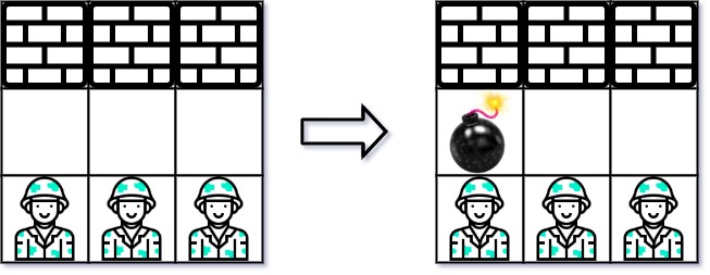
• Given an m x n matrix grid where each cell is either a wall 'W', an enemy 'E' or empty '0', return the maximum enemies you can kill using one bomb. You can only place the bomb in an empty cell.

• The bomb kills all the enemies in the same row and column from the planted point until it hits the wall since it is too strong to be destroyed.

• Example 1:

Input: grid = [["0","E","0","0"],["E","0","W","E"],["0","E","0","0"]]
Output: 3

• Example 2:

Input: grid = [["W","W","W"],["0","0","0"],["E","E","E"]]
Output: 1

• Constraints:
  • m == grid.length
  • n == grid[i].length
  • 1 <= m, n <= 500
  • grid[i][j] is either 'W', 'E', or '0'.
• See problem on LeetCode.

Solution: Brute-force

• Intuition:

  • Arguably the most intuitive solution is to try out all empty cells, i.e. placing a bomb on each empty to see how many enemies it will kill.

  

  • As naïve as it might sound, this approach can pass the test on the online judge.

• Algorithm:

  • We enumerate each cell in the grid from left to right and from top to bottom. For each empty cell, we calculate how many enemies it will kill if we place a bomb on the cell.
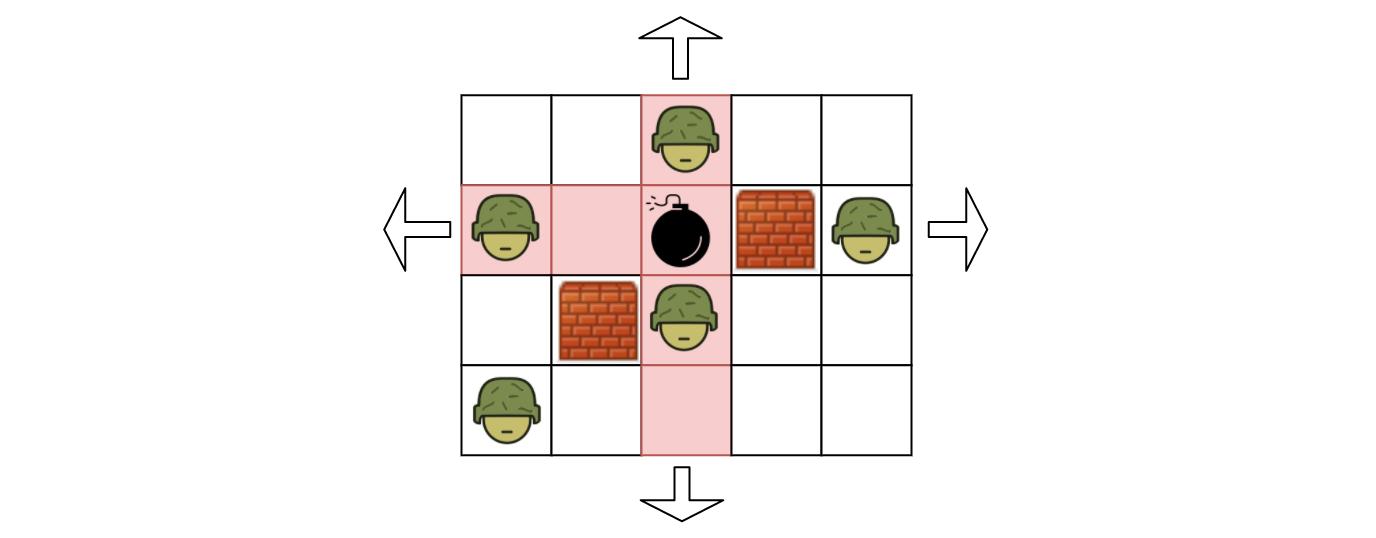
  • We define a function named killEnemies(row, col) which returns the number of enemies we kill if we place a bomb on the coordinate of (row, col).
  • In order to implement the killEnemies(row, col) function, starting from the position of empty cell (row, col), we move away from the cell in four directions (i.e. left, right, up, down), until we run into a wall or the boundary of the grid.
  • At the end of enumeration, we return the maximum value among all the return values of killEnemies(row, col).

class Solution:
    def maxKilledEnemies(self, grid: List[List[str]]) -> int:
        if len(grid) == 0:
            return 0

        rows, cols = len(grid), len(grid[0])

        # find the killed enemy count given a row, col
        def killEnemies(row, col):
            enemy_count = 0
            # killed enemies along a row
            # consider all rows apart from the current row
            row_ranges = [range(row - 1, -1, -1), range(row + 1, rows, 1)]
            for row_range in row_ranges:
                for r in row_range:
                    if grid[r][col] == 'W':
                        break
                    elif grid[r][col] == 'E':
                        enemy_count += 1

            # killed enemies along a col
            # consider all rows apart from the current col
            col_ranges = [range(col - 1, -1, -1), range(col + 1, cols, 1)]
            for col_range in col_ranges:
                for c in col_range:
                    if grid[row][c] == 'W':
                        break
                    elif grid[row][c] == 'E':
                        enemy_count += 1

            return enemy_count

        # find the max
        # note that we do not accumulate all results to a list to find the max
        # but instead compare the current count with the current max as below 
        max_count = 0
        for row in range(0, rows):
            for col in range(0, cols):
                if grid[row][col] == '0':
                    max_count = max(max_count, killEnemies(row, col))

        return max_count

Complexity

• Time: \(\mathcal{O}\big(W \cdot H \cdot (W+H)\big)\) where \(W\) is the width of the grid and \(H\) is the height of the grid.

  • We run an iteration over each element in the grid. In total, the number of iterations would be \(W \cdot H\).

  • Within each iteration, we need to calculate how many enemies we will kill if we place a bomb on the given cell. In the worst case where there is no wall in the grid, we need to check \((W - 1 + H - 1)\) number of cells (all cells in the row/column apart from the cell itself).

  • To sum up, in the worst case where all cells are empty, the number of checks we need to perform would be W \cdot H \cdot (W-1+H-1)W⋅H⋅(W−1+H−1). Hence the overall time complexity of the algorithm is \(\mathcal{O}\big(W \cdot H \cdot (W+H)\big)\).

• Space: \(\mathcal{O}(1)\).

  • The size of the variables that we used in the algorithm is constant, regardless of the input.

Solution: Dynamic Programming

• Intuition:
  • As one might notice in the above brute-force approach, there are some redundant calculations during the iteration. More specifically, for any row or column that does not have any wall in-between, the number of enemies that we can kill remains the same for any empty cell on that particular row or column. While in our brute-force approach, we would iterate the same row or column over and over, regardless the situation of the cells.
  • In order to reduce or even eliminate the redundant calculation, one might recall one of the well-known techniques called Dynamic Programming. The basic principle of dynamic programming is that we store the immediate results which are intended to be reused later, to avoid recalculation.
  • However, the key to apply the dynamic programming technique depends on how we can decompose the problem into a set of subproblems. The solutions of subproblems would then be kept as intermediate results, in order to calculate the final result.
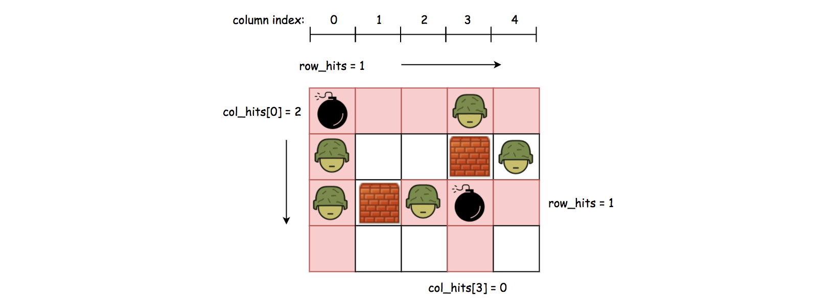
  • Now let us get back to our problem. Given an empty cell located at (row, col), if we place a bomb on the cell, as we know, its influence zone would extend over the same row and column. Let us define the number of enemies that the bomb kills as total_hits, and the number of enemies it kills along the row and column as row_hits and col_hits respectively. As one might figure, we can obtain the equation of total_hits = row_hits + col_hits.
  • It now boils down to how we calculate the row_hits and col_hits for each cell, and moreover how we can reuse the results.
  • Let us take a look at some examples.

  

  • In order to calculate the row_hits, we can break it down into two cases:
    • Case 1: if the cell is situated at the beginning of the row, we then can scan the entire row until we run into a wall or the boundary of the grid. The number of enemies that we encounter along the scan would be the value for row_hits. And the row_hits value that we obtained would remain valid until the next obstacle. For example, as we can see the top-left cell in the above graph, its row_hits would be one and it remains valid for the rest of the cells on the same row.
    • Case 2: if the cell is situated right after a wall, which indicates that the previous row_hits that we calculated becomes invalid. As a result, we need to recalculate the value for row_hits starting from this cell. For example, for the enemy cell that is located on the column of index 2, right before the cell, there is a wall, which invalidates the previous row_hits value. As a result, we run another scan starting from this cell, to calculate the row_hits value.
  • We can calculate the value for col_hits in the same spirit, but with one small difference.
    • For the row_hits value, it suffices to use one variable for all the cells on the same row, since we iterate over the grid from left to right and we don’t need to memorize the row_hits value for the previous row.
    • As for the col_hits value, we need to use an array to keep track of all the col_hits values, since we need to go over all the columns for each row.
• Algorithm:
  • The overall algorithm is rather similar with the brute-force approach, where we still run an iteration over each cell in the grid.
  • Rather than recalculating the hits for each cell, we store the intermediate results such as row_hits and col_hits and reuse them whenever possible.

class Solution:
    def maxKilledEnemies(self, grid: List[List[str]]) -> int:
        if len(grid) == 0:
            return 0

        rows, cols = len(grid), len(grid[0])

        max_count = 0
        row_hits = 0
        col_hits = [0] * cols

        for row in range(0, rows):
            for col in range(0, cols):
                # reset the hits on the row, if necessary.
                if col == 0 or grid[row][col - 1] == 'W':
                    row_hits = 0
                    for k in range(col, cols):
                        if grid[row][k] == 'W':
                            # stop the scan when we hit the wall.
                            break
                        elif grid[row][k] == 'E':
                            row_hits += 1

                # reset the hits on the col, if necessary.
                if row == 0 or grid[row - 1][col] == 'W':
                    col_hits[col] = 0
                    for k in range(row, rows):
                        if grid[k][col] == 'W':
                            break
                        elif grid[k][col] == 'E':
                            col_hits[col] += 1

                # count the hits for each empty cell.
                if grid[row][col] == '0':
                    total_hits = row_hits + col_hits[col]
                    max_count = max(max_count, total_hits)

        return max_count

Complexity

• Time: \(\mathcal{O}(W \cdot H)\) where Let \(W\) be the width of the grid and \(H\) be the height of the grid.

  • One might argue that the time complexity should be \(\mathcal{O}\big(W \cdot H \cdot (W + H)\big)\), judging from the detail that we run nested loop for each cell in grid. If this is the case, then the time complexity of our dynamic programming approach would be the same as the brute-force approach. Yet this is contradicted to the fact that by applying the dynamic programming technique we reduce the redundant calculation.
  • To estimate overall time complexity, let us take another perspective. Concerning each cell in the grid, we assert that it would be visited exactly three times. The first visit is the case where we iterate through each cell in the grid in the outer loop. The second visit would occur when we need to calculate the row_hits that involves with the cell. And finally the third visit would occur when we calculate the value of col_hits that involves with the cell.
  • Based on the above analysis, we can say that the overall time complexity of this dynamic programming approach is \(\mathcal{O}(3 \cdot W \cdot H) = \mathcal{O}(W \cdot H)\).

• Space: \(\mathcal{O}(W)\)

  • In general, with the dynamic programming approach, we gain in terms of time complexity by trading off some space complexity.

  • In our case, we allocate some variables to hold the intermediates results, namely row_hits and col_hits[*]. Therefore, the overall space complexity of the algorithm is \mathcal{O}(W)O(W), where WW is the number of columns in the grid.

[733/Easy] Flood Fill

Problem

• An image is represented by an m x n integer grid image where image[i][j] represents the pixel value of the image.

• You are also given three integers sr, sc, and newColor. You should perform a flood fill on the image starting from the pixel image[sr][sc].

• To perform a flood fill, consider the starting pixel, plus any pixels connected 4-directionally to the starting pixel of the same color as the starting pixel, plus any pixels connected 4-directionally to those pixels (also with the same color), and so on. Replace the color of all of the aforementioned pixels with newColor.

• Return the modified image after performing the flood fill.

• Example 1:

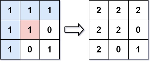
Input: image = [[1,1,1],[1,1,0],[1,0,1]], sr = 1, sc = 1, newColor = 2
Output: [[2,2,2],[2,2,0],[2,0,1]]
Explanation: From the center of the image with position (sr, sc) = (1, 1) (i.e., the red pixel), all pixels connected by a path of the same color as the starting pixel (i.e., the blue pixels) are colored with the new color.
Note the bottom corner is not colored 2, because it is not 4-directionally connected to the starting pixel.

• Example 2:

Input: image = [[0,0,0],[0,0,0]], sr = 0, sc = 0, newColor = 2
Output: [[2,2,2],[2,2,2]]

• See problem on LeetCode.

Solution: DFS

• Intuition:
  • We perform the algorithm explained in the problem description: paint the starting pixels, plus adjacent pixels of the same color, and so on.
• Algorithm:
  • Say color is the color of the starting pixel. Let’s floodfill the starting pixel: we change the color of that pixel to the new color, then check the 4 neighboring pixels to make sure they are valid pixels of the same color, and of the valid ones, we floodfill those, and so on.
  • We can use a function dfs to perform a floodfill on a target pixel.

class Solution:
    def floodFill(self, image: List[List[int]], sr: int, sc: int, newColor: int) -> List[List[int]]:
        # Getting image sizes
        R, C = len(image), len(image[0])
        color = image[sr][sc]
        
        # base case
        if color == newColor: 
            return image
   
        def dfs(r, c):
            if image[r][c] == color:
                # Only other option is that the pixel is in bounds and == oldColor                
                image[r][c] = newColor
                
                # Call dfs on all adjacent pixels
                if r >= 1: 
                    dfs(r-1, c)
                
                if r+1 < R: 
                    dfs(r+1, c)
                
                if c >= 1: 
                    dfs(r, c-1)
                
                if c+1 < C: 
                    dfs(r, c+1)

        # if newColor is not equal to the current color at (sr, sc) try to flood fill
        dfs(sr, sc)
        
        # All applicable pixels have been changed, return image
        return image

Complexity

• Time: \(O(n)\), where \(n\) is the number of pixels in the image. We might process every pixel in the worst case.
• Space: \(O(n)\) for callstacks.

[827/Hard] Making A Large Island

Problem

• You are given an n x n binary matrix grid. You are allowed to change at most one 0 to be 1.

• Return the size of the largest island in grid after applying this operation.

• An island is a 4-directionally connected group of 1s.

• Example 1:

Input: grid = [[1,0],[0,1]]
Output: 3
Explanation: Change one 0 to 1 and connect two 1s, then we get an island with area = 3.

• Example 2:

Input: grid = [[1,1],[1,0]]
Output: 4
Explanation: Change the 0 to 1 and make the island bigger, only one island with area = 4.

• Example 3:

Input: grid = [[1,1],[1,1]]
Output: 4
Explanation: Can't change any 0 to 1, only one island with area = 4.

• Constraints:
  • n == grid.length
  • n == grid[i].length
  • 1 <= n <= 500
  • grid[i][j] is either 0 or 1.
• See problem on LeetCode.

Solution: Naive DFS

• Intuition:
  • For each 0 in the grid, let’s temporarily change it to a 1, then count the size of the group from that square.
• Algorithm:
  • For each 0, change it to a 1, then do a depth first search to find the size of that component. The answer is the maximum size component found.
  • Of course, if there is no 0 in the grid, then the answer is the size of the whole grid.

class Solution(object):
    def largestIsland(self, grid):
        N = len(grid)

        def check(r, c):
            seen = {(r, c)}
            stack = [(r, c)]
            while stack:
                r, c = stack.pop()
                for nr, nc in ((r-1, c), (r, c-1), (r+1, c), (r, c+1)):
                    if (nr, nc) not in seen and 0 <= nr < N and 0 <= nc < N and grid[nr][nc]:
                        stack.append((nr, nc))
                        seen.add((nr, nc))
            return len(seen)

        ans = 0
        has_zero = False
        for r, row in enumerate(grid):
            for c, val in enumerate(row):
                if val == 0:
                    has_zero = True
                    grid[r][c] = 1
                    ans = max(ans, check(r, c))
                    grid[r][c] = 0

        return ans if has_zero else N*N

Complexity

• Time: \(O(N^4)\), where \(N\) is the length and width of the grid.
• Space: \(O(N^2)\), the additional space used in the depth first search by stack and seen.

Solution: Backtracking/DFS

• area maps the id of an island to its area, and address maps each land piece to the id of the island that it belongs to.

class Solution:
    def largestIsland(self, grid: List[List[int]]) -> int:
        N = len(grid)
        DIRECTIONS = [(-1, 0), (0, -1), (0, 1), (1, 0)]
        
        address = {}
        def dfs(row, column, island_id):
            queue = deque([(row, column, island_id)])
            visited.add((row, column))
            area = 1
            
            while queue: 
                row, column, island_id = queue.pop()
                address[(row, column)] = island_id
                for direction in DIRECTIONS:
                    r, c = row + direction[0], column + direction[1]
                    if r in range(N) and c in range(N) and grid[r][c] == 1 and (r, c) not in visited:
                        queue.append((r, c, island_id))
                        visited.add((r, c))
                        area += 1
            return area
        
        visited = set()
        area = {}
        island_id = 0
        for row in range(N):
            for column in range(N):
                if grid[row][column] == 1 and (row, column) not in visited:
                    area[island_id] = dfs(row, column, island_id)
                    island_id += 1
                    
        if len(address.keys()) == N**2: 
            return N**2   
        
        largest_area = 1
        for row in range(N):
            for column in range(N):
                if grid[row][column] == 1: 
                    continue
                    
                neighbours = set()
                large_area = 1
                
                for direction in DIRECTIONS:
                    r, c = row + direction[0], column + direction[1]
                    if r in range(N) and c in range(N) and grid[r][c] == 1 and address[(r, c)] not in neighbours:
                        neighbours.add(address[(r, c)])
                        large_area += area[address[(r, c)]]
                
                largest_area = max(largest_area, large_area)
                
        return largest_area

• Cleaner:

class Solution:
    def largestIsland(self, grid: List[List[int]]) -> int:
        m, n = len(grid), len(grid[0])
        coloredIsland = [[0 for _ in range(n)] for _ in range(m)]
        islandSize = collections.defaultdict(int)
        color = 1
        largest = 0
        
        for r in range(m):
            for c in range(n):
                if grid[r][c] == 1 and coloredIsland[r][c] == 0: # (r, c) is island and not colored yet
                    self.dfsColorIsland(grid, coloredIsland, islandSize, color, r, c)
                    color += 1
                    largest = max(largest, islandSize[coloredIsland[r][c]])

        for r in range(m):
            for c in range(n):
                if grid[r][c] == 0:
                    largest = max(largest, self.countNewIsland(coloredIsland, islandSize, r, c))

        return largest        
    
    def dfsColorIsland(self, grid, coloredIsland, islandSize, color, row, col):
        coloredIsland[row][col] = color
        islandSize[color] += 1
        
        m, n = len(grid), len(grid[0])
        for r, c in [(row-1, col), (row+1, col), (row, col-1), (row, col+1)]:
            if 0 <= r < m and 0 <= c < n and grid[r][c] == 1 and coloredIsland[r][c] == 0:
                self.dfsColorIsland(grid, coloredIsland, islandSize, color, r, c)
    
    def countNewIsland(self, coloredIsland, islandSize, row, col):
        total = 1
        visited = set([0])
        
        m, n = len(coloredIsland), len(coloredIsland[0])
        for r, c in [(row-1, col), (row+1, col), (row, col-1), (row, col+1)]:
            if 0 <= r < m and 0 <= c < n and coloredIsland[r][c] not in visited:
                visited.add(coloredIsland[r][c])
                total += islandSize[coloredIsland[r][c]]

        return total

Complexity

• Time: \(O(n^2)\)
• Space: \(O(n^2)\)

Solution: Component Sizes

• Intuition:
  • As in the previous solution, we check every 0. However, we also store the size of each group, so that we do not have to use depth-first search to repeatedly calculate the same size.
  • However, this idea fails when the 0 touches the same group. For example, consider grid = [[0,1],[1,1]]. The answer is 4, not 1 + 3 + 3, since the right neighbor and the bottom neighbor of the 0 belong to the same group.
  • We can remedy this problem by keeping track of a group id (or index), that is unique for each group. Then, we’ll only add areas of neighboring groups with different ids.
• Algorithm:
  • For each group, fill it with value index and remember it’s size as area[index] = dfs(...).
  • Then for each 0, look at the neighboring group ids seen and add the area of those groups, plus 1 for the 0 we are toggling. This gives us a candidate answer, and we take the maximum.
  • To solve the issue of having potentially no 0, we take the maximum of the previously calculated areas.

class Solution:
    def largestIsland(self, grid: List[List[int]]) -> int:
        N = len(grid)

        def neighbors(r, c):
            for nr, nc in ((r-1, c), (r+1, c), (r, c-1), (r, c+1)):
                if 0 <= nr < N and 0 <= nc < N:
                    yield nr, nc

        def dfs(r, c, index):
            ans = 1
            grid[r][c] = index
            for nr, nc in neighbors(r, c):
                if grid[nr][nc] == 1:
                    ans += dfs(nr, nc, index)
            return ans

        area = {}
        index = 2
        for r in range(N):
            for c in range(N):
                if grid[r][c] == 1:
                    area[index] = dfs(r, c, index)
                    index += 1

        ans = max(area.values() or [0])
        for r in range(N):
            for c in range(N):
                if grid[r][c] == 0:
                    seen = {grid[nr][nc] for nr, nc in neighbors(r, c) if grid[nr][nc] > 1}
                    ans = max(ans, 1 + sum(area[i] for i in seen))
        return ans

Complexity

• Time: \(O(N^2)\), where \(N\) is the length and width of the grid.
• Space: \(O(N^2)\), the additional space used in the depth first search by area.

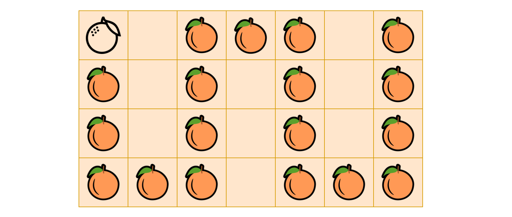
[994/Medium] Rotting Oranges

Problem

• You are given an m x n grid where each cell can have one of three values:

  • 0 representing an empty cell,
  • 1 representing a fresh orange, or
  • 2 representing a rotten orange.

• Every minute, any fresh orange that is 4-directionally adjacent to a rotten orange becomes rotten.

• Return the minimum number of minutes that must elapse until no cell has a fresh orange. If this is impossible, return -1.

• Example 1:

Input: grid = [[2,1,1],[1,1,0],[0,1,1]]
Output: 4

• Example 2:

Input: grid = [[2,1,1],[0,1,1],[1,0,1]]
Output: -1
Explanation: The orange in the bottom left corner (row 2, column 0) is never rotten, because rotting only happens 4-directionally.

• Example 3:

Input: grid = [[0,2]]
Output: 0
Explanation: Since there are already no fresh oranges at minute 0, the answer is just 0.

• Constraints:
  • m == grid.length
  • n == grid[i].length
  • 1 <= m, n <= 10
  • grid[i][j] is 0, 1, or 2.
• See problem on LeetCode.

Solution: BFS

• Intuition:
  • This is yet another 2D traversal problem. As we know, the common algorithmic strategies to deal with these problems would be Breadth-First Search (BFS) and Depth-First Search (DFS).
  • As suggested by its name, the BFS strategy prioritizes the breadth over depth, i.e. it goes wider before it goes deeper. On the other hand, the DFS strategy prioritizes the depth over breadth.
  • The choice of strategy depends on the nature of the problem. Though sometimes, they are both applicable for the same problem. In addition to 2D grids, these two algorithms are often applied to problems associated with tree or graph data structures as well.
  • In this problem, one can see that BFS would be a better fit.

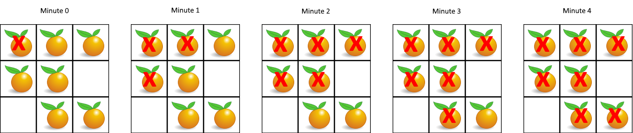
    Because the process of rotting could be explained perfectly with the BFS procedure, i.e. the rotten oranges will contaminate their neighbors first, before the contamination propagates to other fresh oranges that are farther away.

  • However, it would be more intuitive to visualize the rotting process with a graph data structure, where each node represents a cell and the edge between two nodes indicates that the given two cells are adjacent to each other.

  

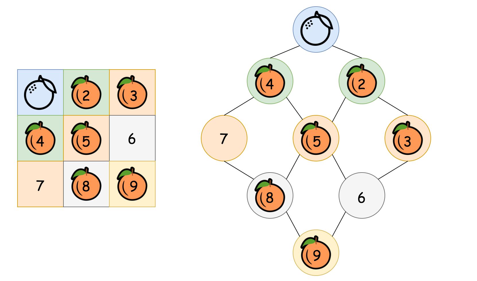
  • In the above graph, as we can see, starting from the top rotten orange, the contamination would propagate layer by layer (or level by level), until it reaches the farthest fresh oranges. The number of minutes that are elapsed would be equivalent to the number of levels in the graph that we traverse during the propagation.
• Algorithm:
  • One of the most distinguished code patterns in BFS algorithms is that often we use a queue data structure to keep track of the candidates that we need to visit during the process.
  • The main algorithm is built around a loop iterating through the queue. At each iteration, we pop out an element from the head of the queue. Then we do some particular process with the popped element. More importantly, we then append neighbors of the popped element into the queue, to keep the BFS process running.

class Solution:
    def orangesRotting(self, grid: List[List[int]]) -> int:

        fresh, rotten = set(), deque()

        # iterate through the grid to get all the fresh and rotten oranges
        for row in range(len(grid)):
            for col in range(len(grid[0])):
                # if we see a fresh orange, put its position in fresh
                if grid[row][col] == 1:
                    fresh.add((row, col))

                # if we see a rotten orange, put its position in rotten
                elif grid[row][col] == 2:
                    rotten.append((row, col))

        minutes = 0
        while fresh and rotten:
            minutes += 1

            # iterate through rotten, popping off the (row, col) that's currently in rotten
            # we don't touch the newly added (row, col) that are added during the loop until the next loop
            for rot in range(len(rotten)):
                row, col = rotten.popleft()

                for direction in ((row - 1, col), (row + 1, col), (row, col - 1), (row, col + 1)):
                    if direction in fresh:
                        # if the (row, col) is in fresh, remove it then add it to rotten
                        fresh.remove(direction)
                        # we will perform 4-directional checks on each (row, col)
                        rotten.append(direction)
    
        # if fresh is not empty, then there is an orange we were not able to reach 4-directionally   print(rotten)
        return -1 if fresh else minutes

Complexity

• Time: \(O(m * n)\)
• Space: \(O(m * n)\)

Solution: BFS with counter for fresh

• The above solution uses a list for book-keeping fresh, let’s use a counter:

from collections import deque
class Solution:
    def orangesRotting(self, grid: List[List[int]]) -> int:
        queue = deque()

        # Step 1). build the initial set of rotten oranges
        fresh_oranges = 0
        ROWS, COLS = len(grid), len(grid[0])
        for r in range(ROWS):
            for c in range(COLS):
                if grid[r][c] == 2:
                    queue.append((r, c))
                elif grid[r][c] == 1:
                    fresh_oranges += 1

        # Mark the round / level, _i.e_ the ticker of timestamp
        queue.append((-1, -1))

        # Step 2). start the rotting process via BFS
        minutes_elapsed = -1
        directions = [(-1, 0), (0, 1), (1, 0), (0, -1)]
        
        while queue:
            row, col = queue.popleft()
            if row == -1:
                # We finish one round of processing
                minutes_elapsed += 1
                if queue:  # to avoid the endless loop
                    queue.append((-1, -1))
            else:
                # this is a rotten orange
                # then it would contaminate its neighbors
                for d in directions:
                    neighbor_row, neighbor_col = row + d[0], col + d[1]
                    if ROWS > neighbor_row >= 0 and COLS > neighbor_col >= 0:
                        if grid[neighbor_row][neighbor_col] == 1:
                            # this orange would be contaminated
                            grid[neighbor_row][neighbor_col] = 2
                            fresh_oranges -= 1
                            # this orange would then contaminate other oranges
                            queue.append((neighbor_row, neighbor_col))

        # return elapsed minutes if no fresh orange left
        return minutes_elapsed if fresh_oranges == 0 else -1

• In the above implementations, we applied some tricks to further optimize both the time and space complexities.
  • Usually in BFS algorithms, we keep a visited table which records the visited candidates. The visited table helps us to avoid repetitive visits.
  • But as one notices, rather than using the visited table, we reuse the input grid to keep track of our visits, i.e. we were altering the status of the input grid in-place.
  • This in-place technique reduces the memory consumption of our algorithm. Also, it has a constant time complexity to check the current status (i.e. array access, grid[row][col]), rather than referring to the visited table which might be of constant time complexity as well (e.g. hash table) but in reality could be slower than array access.
  • We use a delimiter (i.e. (row=-1, col=-1)) in the queue to separate cells on different levels. In this way, we only need one queue for the iteration. As an alternative, one can create a queue for each level and alternate between the queues, though technically the initialization and the assignment of each queue could consume some extra time.

Complexity

• Time: \(O(m * n)\), where \(m\) and \(n\) are the rows and cols in the grid.
  • First, we scan the grid to find the initial values for the queue, which would take \(O(n)\) time.
  • Then we run the BFS process on the queue, which in the worst case would enumerate all the cells in the grid once and only once.
  • Therefore, it takes \(O(n)\) time. Thus combining the above two steps, the overall time complexity would be \(O(n + n) = O(n)\).
• Space: \(O(m * n)\), where \(m\) and \(n\) are the rows and cols in the grid.
  • In the worst case, the grid is filled with rotten oranges. As a result, the queue would be initialized with all the cells in the grid.
  • By the way, normally for BFS, the main space complexity lies in the process rather than the initialization. For instance, for a BFS traversal in a tree, at any given moment, the queue would hold no more than 2 levels of tree nodes. Therefore, the space complexity of BFS traversal in a tree would depend on the width of the input tree.

Solution: In-place BFS

• Intuition:
  • Although there is no doubt that the best strategy for this problem is BFS, here’s an implementation of BFS with constant space complexity \(O(1)\).
  • As one might recall from the previous BFS implementation, its space complexity is mainly due to the queue that we were using to keep the order for the visits of cells. In order to achieve \mathcal{O}(1)O(1) space complexity, we then need to eliminate the queue in the BFS.

    The secret in doing BFS traversal without a queue lies in the technique called in-place algorithm, which transforms input to solve the problem without using auxiliary data structure.

  • Actually, we have already had a taste of in-place algorithm in the previous implementation of BFS, where we directly modified the input grid to mark the oranges that turn rotten, rather than using an additional visited table.
  • How about we apply the in-place algorithm again, but this time for the role of the queue variable in our previous BFS implementation?

    The idea is that at each round of the BFS, we mark the cells to be visited in the input grid with a specific timestamp.

  • By round, we mean a snapshot in time where a group of oranges turns rotten.

• Algorithm:

  

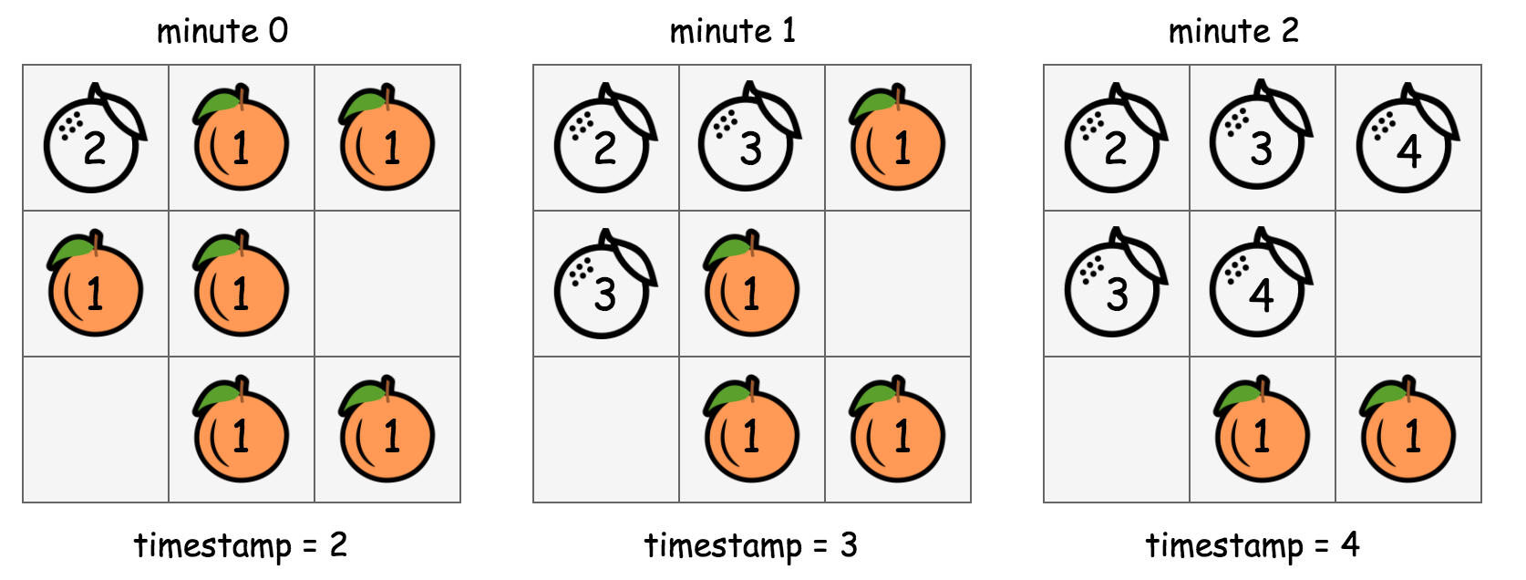
  • In the above graph, we show how we manipulate the values in the input grid in-place in order to run the BFS traversal.
    • Starting from the beginning (with timestamp=2), the cells that are marked with the value 2 contain rotten oranges. From this moment on, we adopt a rule stating as “the cells that have the value of the current timestamp (i.e. 2) should be visited at this round of BFS.”.
    • For each of the cell that is marked with the current timestamp, we then go on to mark its neighbor cells that hold a fresh orange with the next timestamp (i.e. timestamp += 1). This in-place modification serves the same purpose as the queue variable in the previous BFS implementation, which is to select the candidates to visit for the next round.
    • At this moment, we should have timestamp=3, and meanwhile we also have the cells to be visited at this round marked out. We then repeat the above step (2) until there is no more new candidates generated in the step (2) (i.e. the end of BFS traversal).
  • To summarize, the above algorithm is still a BFS traversal in a 2D grid. But rather than using a queue data structure to keep track of the visiting order, we applied an in-place algorithm to serve the same purpose as a queue in a more classic BFS implementation.

class Solution(object):
    def orangesRotting(self, grid):
        ROWS, COLS = len(grid), len(grid[0])

        # run the rotting process, by marking the rotten oranges with the timestamp
        directions = [(-1, 0), (0, 1), (1, 0), (0, -1)]
        
        def runRottingProcess(timestamp):
            # flag to indicate if the rotting process should be continued
            to_be_continued = False
            for row in range(ROWS):
                for col in range(COLS):
                    if grid[row][col] == timestamp:
                        # current contaminated cell
                        for d in directions:
                            n_row, n_col = row + d[0], col + d[1]
                            if ROWS > n_row >= 0 and COLS > n_col >= 0:
                                if grid[n_row][n_col] == 1:
                                    # this fresh orange would be contaminated next
                                    grid[n_row][n_col] = timestamp + 1
                                    to_be_continued = True
            return to_be_continued

        timestamp = 2
        while runRottingProcess(timestamp):
            timestamp += 1
            
        # end of process, to check if there are still fresh oranges left
        for row in grid:
            for cell in row:
                if cell == 1:  # still got a fresh orange left
                    return -1
                    
        # return elapsed minutes if no fresh orange left
        return timestamp - 2

Complexity

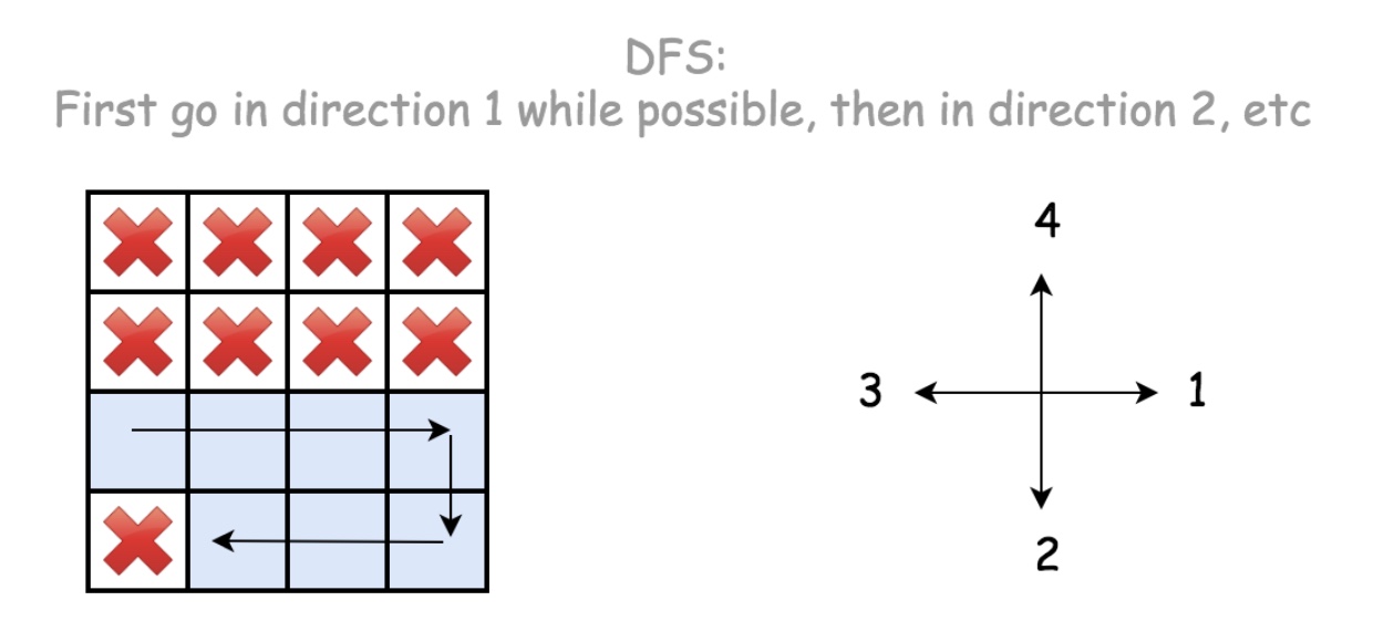
• Time: \(O((m * n)^2)\), where \(m\) and \(n\) are the rows and cols in the grid.
  • In the in-place BFS traversal, for each round of BFS, we would have to iterate through the entire grid.
  • The contamination propagates in 4 different directions. If the orange is well adjacent to each other, the chain of propagation would continue until all the oranges turn rotten.
  • In the worst case, the rotten and the fresh oranges might be arranged in a way that we would have to run the BFS loop over and over again, which could amount to \(\frac{N}{2}\) times which is the longest propagation chain that we might have, i.e. the zigzag walk in a 2D grid as shown in the following graph.

  

  • As a result, the overall time complexity of the in-place BFS algorithm is \(\mathcal{O}(N \cdot \frac{N}{2}) = \mathcal{O}(N^2)\).
• Space: \(O(1)\), the memory usage is constant regardless the size of the input. This is the very point of applying in-place algorithm. Here we trade the time complexity with the space complexity, which is a common scenario in many algorithms.

[1091/Medium] Shortest Path in Binary Matrix

Problem

• Given an n x n binary matrix grid, return the length of the shortest clear path in the matrix. If there is no clear path, return -1.
• A clear path in a binary matrix is a path from the top-left cell (i.e., (0, 0)) to the bottom-right cell (i.e., (n - 1, n - 1)) such that:
  • All the visited cells of the path are 0.
  • All the adjacent cells of the path are 8-directionally connected (i.e., they are different and they share an edge or a corner).

• The length of a clear path is the number of visited cells of this path.

• Example 1:

Input: grid = [[0,1],[1,0]]
Output: 2

• Example 2:

Input: grid = [[0,0,0],[1,1,0],[1,1,0]]
Output: 4

• Example 3:

Input: grid = [[1,0,0],[1,1,0],[1,1,0]]
Output: -1

• See problem on LeetCode.

Solution: BFS

• Since it’s BFS, we can securely set the visited grid as non-empty to avoid revisiting.

def shortestPathBinaryMatrix(grid):
    n = len(grid)
    
    if grid[0][0] or grid[n-1][n-1]:
        return -1
    q = [(0, 0, 1)]
    
    grid[0][0] = 1
    for i, j, d in q:
        if i == n-1 and j == n-1: return d
        for x, y in ((i-1,j-1), (i-1,j), (i-1,j+1), (i,j-1), (i,j+1), (i+1,j-1), (i+1,j), (i+1,j+1)):
            if 0 <= x < n and 0 <= y < n and not grid[x][y]:
                grid[x][y] = 1
                q.append((x, y, d+1))
                
    return -1

Solution: BFS + Deque

• A more general approach with deque without corrupting the input:

def shortestPathBinaryMatrix(self, grid: List[List[int]]) -> int:
        n = len(grid)
        if grid[0][0] or grid[n-1][n-1]:
          return -1
          
        dirs = [[1,0], [-1,0], [0,1], [0,-1], [-1,-1], [1,1], [1,-1], [-1,1]]
        seen = set()
        queue = collections.deque([(0,0,1)]) # indice, dist
        seen.add((0,0))
        while queue:
            i, j, dist = queue.popleft()
            
            if i == n -1 and j == n - 1:
                return dist
                
            for d1, d2 in dirs: 
                x, y = i + d1, j + d2
                if 0 <= x < n and 0 <= y < n:
                    if (x,y) not in seen and grid[x][y] == 0:
                        seen.add((x, y))
                        queue.append((x, y, dist + 1))
                
        return -1

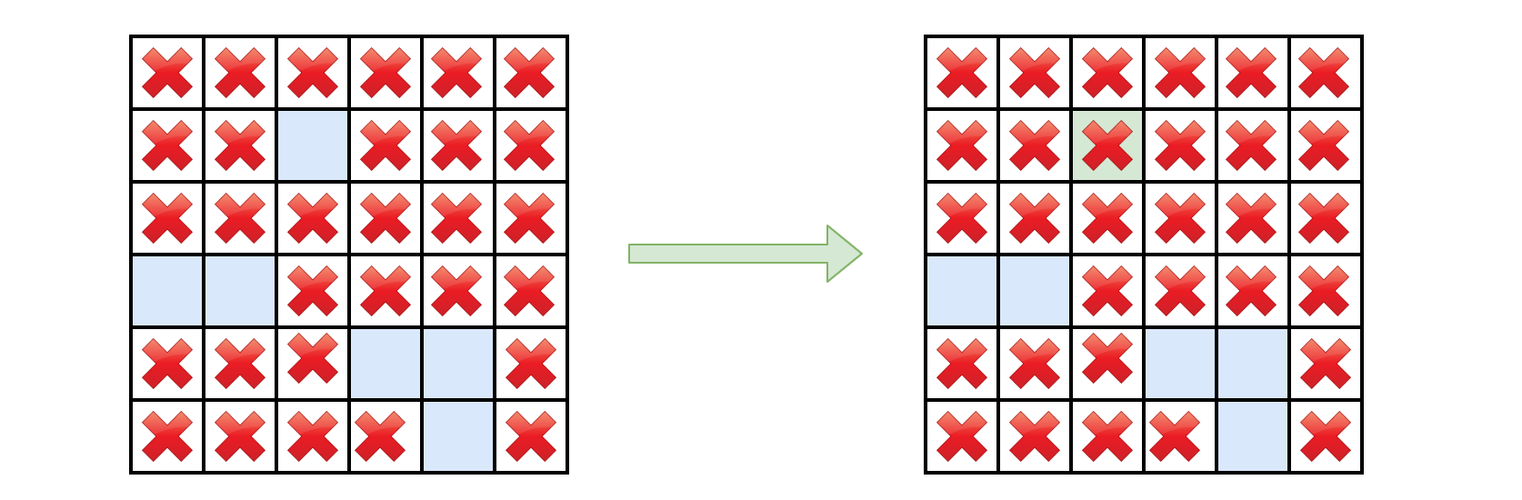
Solution: A* search

Concept

• An A* search is like a breadth-first search, except that in each iteration, instead of expanding the cell with the shortest path from the origin, we expand the cell with the lowest overall estimated path length – this is the distance so far, plus a heuristic (rule-of-thumb) estimate of the remaining distance. As long as the heuristic is consistent, an A* graph-search will find the shortest path. This can be somewhat more efficient than breadth-first-search as we typically don’t have to visit nearly as many cells. Intuitively, an A* search has an approximate sense of direction, and uses this sense to guide it towards the target.

• Example

[
    [0,0,0,1,0,0,1,0],
    [0,0,0,0,0,0,0,0],
    [1,0,0,1,1,0,1,0],
    [0,1,1,1,0,0,0,0],
    [0,0,0,0,0,1,1,1],
    [1,0,1,0,0,0,0,0],
    [1,1,0,0,0,1,0,0],
    [0,0,0,0,0,1,0,0]
]

• With this grid, an A* search will explore only the green cells in this animation:

• Whereas a BFS will visit every cell:

• Implementation
  • We perform an A* search to find the shortest path, then return it’s length, if there is one. Note: I chose to deal with the special case, that the starting cell is a blocking cell, here rather than complicate the search implementation.

class Solution:
    def shortestPathBinaryMatrix(self, grid):
        shortest_path = a_star_graph_search(
            start              = (0, 0), 
            goal_function      = get_goal_function(grid),
            successor_function = get_successor_function(grid),
            heuristic          = get_heuristic(grid)
        )
        if shortest_path is None or grid[0][0] == 1:
            return -1
        else:
            return len(shortest_path)

• A* search function
  • This implementation is somewhat general and will work for other constant-cost search problems, as long as you provide a suitable goal function, successor function, and heuristic.

def a_star_graph_search(
            start,
            goal_function,
            successor_function,
            heuristic
    ):
    visited = set()
    came_from = dict()
    distance = {start: 0}
    frontier = PriorityQueue()
    frontier.add(start)
    while frontier:
        node = frontier.pop()
        if node in visited:
            continue
        if goal_function(node):
            return reconstruct_path(came_from, start, node)
        visited.add(node)
        for successor in successor_function(node):
            frontier.add(
                successor,
                priority = distance[node] + 1 + heuristic(successor)
            )
            if (successor not in distance
                or distance[node] + 1 < distance[successor]):
                distance[successor] = distance[node] + 1
                came_from[successor] = node
    return None

def reconstruct_path(came_from, start, end):
    """
    >>> came_from = {'b': 'a', 'c': 'a', 'd': 'c', 'e': 'd', 'f': 'd'}
    >>> reconstruct_path(came_from, 'a', 'e')
    ['a', 'c', 'd', 'e']
    """
    reverse_path = [end]
    while end != start:
        end = came_from[end]
        reverse_path.append(end)
    return list(reversed(reverse_path))

• Goal function
  • We need a function to check whether we have reached the goal cell:

def get_goal_function(grid):
    """
    >>> f = get_goal_function([[0, 0], [0, 0]])
    >>> f((0, 0))
    False
    >>> f((0, 1))
    False
    >>> f((1, 1))
    True
    """
    M = len(grid)
    N = len(grid[0])
    def is_bottom_right(cell):
        return cell == (M-1, N-1)
    return is_bottom_right

• Successor function
  • We also need a function to find the cells adjacent to the current cell:

def get_successor_function(grid):
    """
    >>> f = get_successor_function([[0, 0, 0], [0, 1, 0], [1, 0, 0]])
    >>> sorted(f((1, 2)))
    [(0, 1), (0, 2), (2, 1), (2, 2)]
    >>> sorted(f((2, 1)))
    [(1, 0), (1, 2), (2, 2)]
    """
    def get_clear_adjacent_cells(cell):
        i, j = cell
        return (
            (i + a, j + b)
            for a in (-1, 0, 1)
            for b in (-1, 0, 1)
            if a != 0 or b != 0
            if 0 <= i + a < len(grid)
            if 0 <= j + b < len(grid[0])
            if grid[i + a][j + b] == 0
        )
    return get_clear_adjacent_cells

• Heuristic
  • The chosen heuristic is simply the distance to the goal in a clear grid of the same size. This turns out to be the maximum of the x-distance and y-distance from the goal. This heuristic is admissible and consistent.

def get_heuristic(grid):
    """
    >>> f = get_heuristic([[0, 0], [0, 0]])
    >>> f((0, 0))
    1
    >>> f((0, 1))
    1
    >>> f((1, 1))
    0
    """
    M, N = len(grid), len(grid[0])
    (a, b) = goal_cell = (M - 1, N - 1)
    def get_clear_path_distance_from_goal(cell):
        (i, j) = cell
        return max(abs(a - i), abs(b - j))
    return get_clear_path_distance_from_goal

• Priority queue
  • The Python standard library provides a heap data structure, but not a priority-queue, so we need to implement one ourselves.

from heapq import heappush, heappop

class PriorityQueue:
    
    def __init__(self, iterable=[]):
        self.heap = []
        for value in iterable:
            heappush(self.heap, (0, value))
    
    def add(self, value, priority=0):
        heappush(self.heap, (priority, value))
    
    def pop(self):
        priority, value = heappop(self.heap)
        return value
    
    def __len__(self):
        return len(self.heap)

• And that’s it.

• Breadth-first search

  • Here is a breadth-first-search implementation, for comparison:

from collections import deque

def breadth_first_search(grid):
    N = len(grid)

    def is_clear(cell):
        return grid[cell[0]][cell[1]] == 0

    def get_neighbours(cell):
        (i, j) = cell
        return (
            (i + a, j + b)
            for a in (-1, 0, 1)
            for b in (-1, 0, 1)
            if a != 0 or b != 0
            if 0 <= i + a < N
            if 0 <= j + b < N
            if is_clear( (i + a, j + b) )
        )

    start = (0, 0)
    goal = (N - 1, N - 1)

    queue = deque()
    if is_clear(start):
        queue.append(start)
    visited = set()
    path_len = {start: 1}

    while queue:
        cell = queue.popleft()
        if cell in visited:
            continue
        if cell == goal:
            return path_len[cell]
        visited.add(cell)
        for neighbour in get_neighbours(cell):
            if neighbour not in path_len:
                path_len[neighbour] = path_len[cell] + 1
            queue.append(neighbour)

    return -1

[1275/Easy] Find Winner on a Tic Tac Toe Game

Problem

• Tic-tac-toe is played by two players A and B on a 3 x 3 grid. The rules of Tic-Tac-Toe are:
  • Players take turns placing characters into empty squares ' '.
  • The first player A always places 'X' characters, while the second player B always places 'O' characters.
  • 'X' and 'O' characters are always placed into empty squares, never on filled ones.
  • The game ends when there are three of the same (non-empty) character filling any row, column, or diagonal.
  • The game also ends if all squares are non-empty.
  • No more moves can be played if the game is over.
• Given a 2D integer array moves where moves[i] = [row_i, col_i] indicates that the i-th move will be played on grid[row_i][col_i]. return the winner of the game if it exists (A or B). In case the game ends in a draw return "Draw". If there are still movements to play return "Pending".

• You can assume that moves is valid (i.e., it follows the rules of Tic-Tac-Toe), the grid is initially empty, and A will play first.

• Example 1:

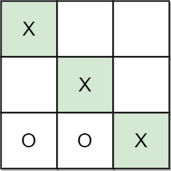
Input: moves = [[0,0],[2,0],[1,1],[2,1],[2,2]]
Output: "A"
Explanation: A wins, they always play first.

• Example 2:

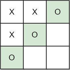
Input: moves = [[0,0],[1,1],[0,1],[0,2],[1,0],[2,0]]
Output: "B"
Explanation: B wins.

• Example 3:

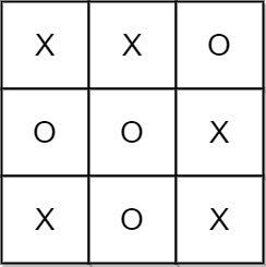
Input: moves = [[0,0],[1,1],[2,0],[1,0],[1,2],[2,1],[0,1],[0,2],[2,2]]
Output: "Draw"
Explanation: The game ends in a draw since there are no moves to make.

• Constraints:
  • 1 <= moves.length <= 9
  • moves[i].length == 2
  • 0 <= rowi, coli <= 2
  • There are no repeated elements on moves.
  • moves follow the rules of tic tac toe.
• See problem on LeetCode.

Solution: Alternate between players, check for the four wining conditions

• Overview:
  • Tic Tac Toe is one of the classic games with pretty simple rules. Two players take turns placing characters on an n by n board. The first player that connects n consecutive characters horizontally, vertically, or diagonally wins the game. Traditionally (and in this problem), the board width is fixed at 3. However, to help demonstrate the efficiency of each approach, we will refer to the board width as n throughout this article.
  • In this problem, we are looking to determine the winner of the game (if one exists). If neither player has won, then we must determine if the game is ongoing or if it has ended in a draw.
  • The most intuitive approach is to check, after each move, if the current player has won, which can be implemented by different methods. Here we introduce two approaches to solve this problem, the first one is the most intuitive one, while the second one has some optimization.
• Approach 1: Brute Force:
  • Intuition:
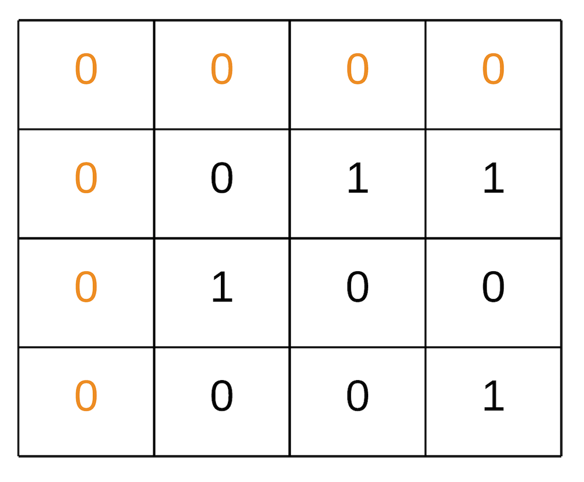
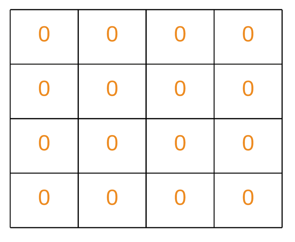
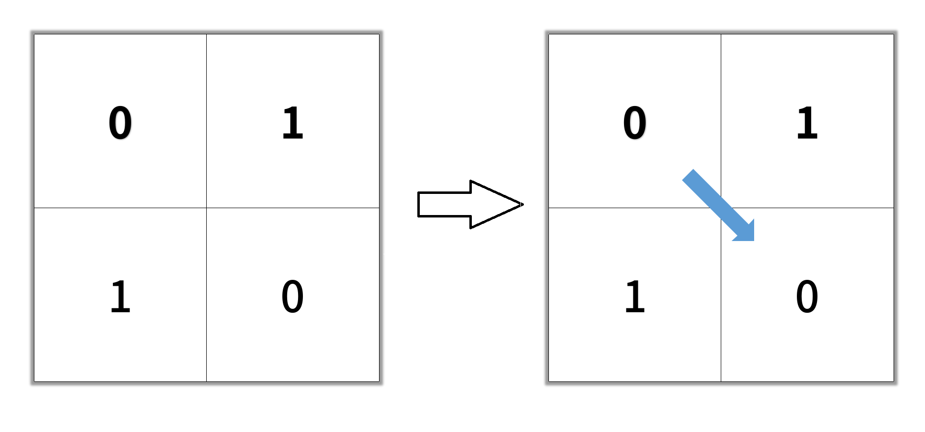
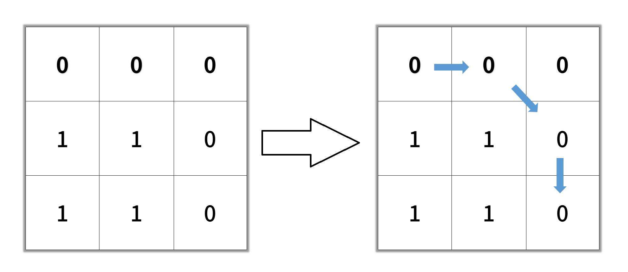
    • Since we have to find if the current player has won, let’s take a look at what the winning conditions are. The figure below illustrates the 4 winning conditions according to the rules.
    • The above diagram shows that a player can win by connecting n consecutive characters in a row, column, diagonal, or anti-diagonal.
    • Then, how do we check if any player has won so far?
    • We can start by creating an n by n grid that represents the original board.
    • Next, let’s take a closer look at the previous winning conditions. Notice that a character located at [row, col] will be on the diagonal when its column index equals its row index, that is row = col. Likewise, a character will be on the anti-diagonal when then the sum of its row index and column index is equal to n - 1, that is row + col = n - 1.
    • Suppose the current player marks the location [row, col], where row and col stand for the row index and column index on board, respectively. If row row or column col has n characters from the same player after this move, then the current player wins.
    • Now, after each move, we can determine if a player has won by checking each row, column, and diagonal. The next question is, how will we determine the result after all moves have been made? We need to find a way to handle cases where neither player wins.
    • If neither player has won after all of the moves have been played, we need to check the length of moves. There are two possibilities: “Draw” if the board is full, meaning the length of moves is n * n, or “Pending” otherwise.
    • Now, we are ready to implement a brute force solution.
• Algorithm:
  • Initialize a 2-dimensional array board of size n by n representing an empty board.
  • For each new move [row, col], mark the relative position board[row][col] on board with the player’s id. Suppose player one’s id is 1, and player two’s id is -1.
  • Then, check if this move meets any of the winning conditions:
    • Check if all cells in the current row are filled with characters from the current player. We traverse the row from column 0 to column n - 1 while keeping the row index constant.
    • Check if all cells in the current column are filled with characters from the current player. We traverse the column from row 0 to row n - 1 while keeping the column index constant.
    • Check if this move is on the diagonal; that is, check if row equals col. If so, traverse the entire diagonal and check if all positions on the diagonal contain characters from this player.
    • Check if this move is on the anti-diagonal; that is, check if row + col equals n - 1. If so, traverse the entire anti-diagonal and check if all positions on the anti-diagonal contain characters from this player.
  • If there is no winner after all of the moves have been played, we will check if the entire board is filled. If so, return “Draw”, otherwise return “Pending”, meaning the game is still on. That is, check if the length of moves equals the number of cells on the n by n board.

class Solution:
    def tictactoe(self, moves: List[List[int]]) -> str:

        # Initialize the board, n = 3 in this problem.
        n = 3
        board = [[0] * n for _ in range(n)]
        
        # Check if any of 4 winning conditions to see if the current player has won.
        def checkRow(row, player_id):
            for col in range(n):
                if board[row][col] != player_id:
                    return False
            return True
        
        def checkCol(col, player_id):
            for row in range(n):
                if board[row][col] != player_id:
                    return False
            return True
        
        def checkDiagonal(player_id):
            for row in range(n):
                if board[row][row] != player_id:
                    return False
            return True
        
        def checkAntiDiagonal(player_id):
            for row in range(n):
                if board[row][n - 1 - row] != player_id:
                    return False
            return True
        
        # Start with player_1.
        player = 1

        for move in moves:
            # extract 
            row, col = move
            board[row][col] = player
            
            # If any of the winning conditions is met, return the current player's id.
            if checkRow(row, player) or checkCol(col, player) or \
            (row == col and checkDiagonal(player)) or \
            (row + col == n - 1 and checkAntiDiagonal(player)):
                return 'A' if player == 1 else 'B'
            
            # If no one wins so far, change to the other player alternatively. 
            # That is from 1 to -1, from -1 to 1.
            player *= -1
            
        # If all moves are completed and there is still no result, we shall check if
        # the grid is full or not. If so, the game ends with draw, otherwise pending.    
        return "Draw" if len(moves) == n * n else "Pending"

Complexity

• Time: \(O(mn)\) where n is the length of the board and m is the length of input moves. Since for every move, we need to traverse the same row, column, diagonal, and anti-diagonal, which takes \(O(n)\) time.
• Space: \(O(n^2)\) for board, since we use an n by n array to record every move.

Solution: Record Each Move

• Intuition:
  • Instead of recording each move in a n by n grid, as we did in the first approach, could we find a more effective way to record the previous moves? The answer is Yes.

    Let’s take a look at the 4 winning conditions again.

  • In the first approach, since we created the board and recorded each move, we had to traverse the entire line to check if all marks were of the same type.

    However, this method stores way more information than we actually need, it also results in an increased time and space complexity.

  • We do not need to know where these marks are located in order to solve the problem. What we do need to know is: after move [row, col], does any row, column, or diagonal meet the winning condition?

    Therefore, we could just record the result of each row and column instead of the position of each move precisely.

  • Now the question becomes: How should we record the result? Let’s take a look at the figure below to find out.

    Notice that there are many unique ways to fill a single row. However, only two cases are considered as a win. Recall that in the first approach, we set the value of players A and B to 1 and -1, respectively. Here we can take advantage of these distinct values again.

  • Suppose we let the value of player A equal 1 and the value of player B equal -1. There are other ways to assign value, but 1 and -1 are the most convenient.
  • Therefore, a player will win if the value of any line equals n or -n. Thus after a move [row, col], we could calculate the value of row row and column col and check if the absolute value equals n. If this move is placed on the diagonal or the anti-diagonal, then we will check if the absolute value of the relative value equals n as well.
  • Thus, we just need to build two arrays to represent the values for each row and column. For instance, rows = [0, 0, 0], represents the initial value of row_1, row_2, and row_3, and the two values diag and anti_diag for value on diagonal and anti-diagonal.
  • To see how this will work, consider the two example moves shown below.
  • After player A plays at [2, 0], we update the value of rows[2] and col[0], since row = 2 and col = 2. Also, because row + col = 2, we will update the value of the anti-diagonal. Since none of these values equals 3 after the update, this means that the game is still on.
  • After player B’s move, we update the value of row[1] and col[1]. Since this character is on both diagonal and anti-diagonal, we update diag and anti_diag as well. We will see that col[1] = -3, which means the current player (player B) has won the game! Thus return B.
• Algorithm:
  • We use two lists, rows and cols of size n, to represent each row and column. We also use two numbers, diag and anti_diag, to represent the diagonal value and anti-diagonal value, respectively.
  • Set the value of player A as 1 and the value of player B as -1.
  • For each new move [row, col], add the player’s value to rows[row] and cols[col]. If [row, col] is on the diagonal or anti-diagonal, then add the player’s value to diag or anti_diag as well.
  • Then, check if this move meets any winning condition:
    • Check if all cells in the current row contain characters from this player. To do so, we just need to check if the absolute value of rows[row] equals n.
    • Check if all cells in the current column contain characters from this player. To do so, we just need to check if the absolute value of cols[col] equals n.
    • Check if this move is on the diagonal; that is if row equals col. If so, check if the absolute value of diag equals n.
    • Check if this move is on the anti-diagonal; that is if row + col equals n - 1. If so, check if the absolute value of anti_diag equals n.
  • If there is no winner after all of the moves have been played, we will check if the entire board is filled. If so, return "Draw", otherwise return "Pending", meaning the game is still on. To determine if the entire board is filled, check if the length of moves equals the number of cells on the n by n board.

class Solution:
    def tictactoe(self, moves: List[List[int]]) -> str:

        # n stands for the size of the board, n = 3 for the current game.
        n = 3

        # use rows and cols to record the value on each row and each column.
        # diag1 and diag2 to record value on diagonal or anti-diagonal.
        rows, cols = [0] * n, [0] * n
        diag = anti_diag = 0
        
        # Two players having value of 1 and -1, player_1 with value = 1 places first.
        player = 1
        
        for row, col in moves:
            
            # Update the row value and column value.
            rows[row] += player
            cols[col] += player
            
            # If this move is placed on diagonal or anti-diagonal, 
            # we shall update the relative value as well.
            if row == col:        
                # row == col: diagonal    
                diag += player
            if row + col == n - 1:
                # row == col: diagonal    
                anti_diag += player
                
            # check if this move meets any of the winning conditions.
            if any(abs(line) == n for line in (rows[row], cols[col], diag, anti_diag)):
                return "A" if player == 1 else "B"
        
            # If no one wins so far, change to the other player alternatively. 
            # That is from 1 to -1, from -1 to 1.
            player *= -1
            
        # If all moves are completed and there is still no result, we shall check if 
        # the grid is full or not. If so, the game ends with draw, otherwise pending.
        return "Draw" if len(moves) == n * n else "Pending"   

Complexity

• Time: \(O(m)\) where m is the length of input moves. For every move, we update the value for a row, column, diagonal, and anti-diagonal. Each update takes constant time. We also check if any of these lines satisfies the winning condition which also takes constant time.
• Space: \(O(n)\) since we use two arrays of size n to record the value for each row and column, and two integers of constant space to record to value for diagonal and anti-diagonal.

[1293/Hard] Shortest Path in a Grid with Obstacles Elimination

Problem

• You are given an m x n integer matrix grid where each cell is either 0 (empty) or 1 (obstacle). You can move up, down, left, or right from and to an empty cell in one step.

• Return the minimum number of steps to walk from the upper left corner (0, 0) to the lower right corner (m - 1, n - 1) given that you can eliminate at most k obstacles. If it is not possible to find such walk return -1.

• Example 1:

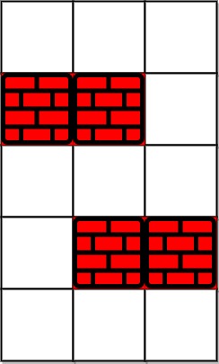
Input: grid = [[0,0,0],[1,1,0],[0,0,0],[0,1,1],[0,0,0]], k = 1
Output: 6
Explanation: 
The shortest path without eliminating any obstacle is 10.
The shortest path with one obstacle elimination at position (3,2) is 6. Such path is (0,0) -> (0,1) -> (0,2) -> (1,2) -> (2,2) -> (3,2) -> (4,2).

• Example 2:

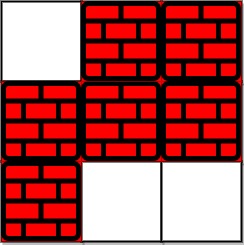
Input: grid = [[0,1,1],[1,1,1],[1,0,0]], k = 1
Output: -1
Explanation: We need to eliminate at least two obstacles to find such a walk.

• Constraints:
  • m == grid.length
  • n == grid[i].length
  • 1 <= m, n <= 40
  • 1 <= k <= m * n
  • - grid[i][j] is either 0 or 1.
  • grid[0][0] == grid[m - 1][n - 1] == 0

Solution: Trivial BFS

• Minimum path problems can be solved by a variety of approaches such as (DP, BFS, Dijkstra, DFS with memo). However, this problem cannot be solved via DP due to a the fact that movement is allowed in all orthogonal directions (a.k.a. all four directions). Also, cost of steps is uniform, hence Dijkstra does not make sense here.

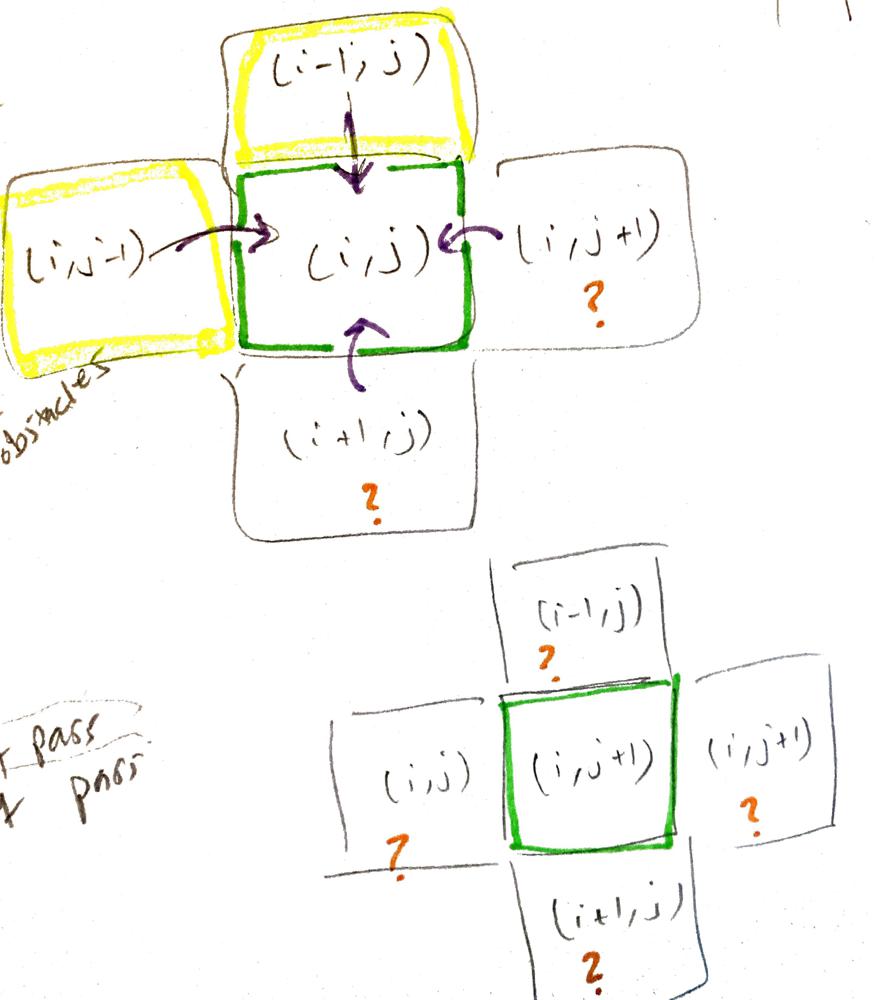
• Another interesting aspect of this problem is the fact that we need to keep track of k (aka. number of passes) as we traverse.
  • This adds a little complexity to the problem and requires some tweaks to the trivial BFS we usually use in uniform grid problems.
  • Why?
    • In trivial BFS, we visit each node only once (we guarantee this behavior by leveraging an visited set).
      • The reason we did that is because we used a queue and we investigated neighbors layer by layer.
      • This means that if a node is seen again, then we are definitely further away than the first time we saw it. Therefore we ignore it right away since its the shortest path is what we are after.
    • However, the fact that we have passes that allows us to ignore obstacles, suggests that we might re-visit the same node via longer route yet with higher number of remaining passes which is something we should not disregard (worthy of exploration). Because it’s very possible for the shorter route with less passes get blocked later on and we never reach target.
• Long story short: We need to allow visiting the same node more than once.
• Here’s our algorithm:
  • Idea: enque neighbor first, then check.
  • The below implementation is slow because I am enquing the neighbors first, then check if target is reached. The next approach speedens things up.

class Solution:
    def shortestPath(self, grid: List[List[int]], k: int) -> int:
        trgtX, trgtY = len(grid)-1, len(grid[0])-1
        if trgtX == trgtY == 0:
            return 0

        if k > trgtX + trgtY: # as if no obstacles
            return trgtX + trgtY # unweighted grid -> shortest distance = all the way to the left + all the way to the right

        from collections import deque
        q = deque()
        q.append((0,0,0,k))
        visited = set()
        # visited.add((0,0,k)) # same cell can be revisited via shorter path and less obstPass
        dirs = [(1,0), (0,1), (-1,0), (0,-1)]
        while q:
            x, y, r, obsPass = q.popleft()

            if (x,y) == (trgtX, trgtY): # trgt reached
                return r

            visited.add((x, y, obsPass))

            for dir in dirs:
                newX, newY = x+dir[0], y+dir[1]
                if newX >= 0 and newX <= trgtX and newY >= 0 and newY <= trgtY:   
                    if grid[newX][newY] == 1: # obstacle
                        if (newX, newY, obsPass-1) not in visited:
                            if obsPass:
                                q.append((newX, newY, r+1, obsPass-1))
                    else:
                        if (newX, newY, obsPass) not in visited:
                            q.append((newX, newY, r+1, obsPass))

        return -1

Complexity

• Time: \(O(kmn)\) since we are allowing the same node to be visited again if \(k\) is different.

Solution: Enhanced BFS

• Unlike the first approach, here the goal test is applied upon generation rather than expansion
• Refer Artificial Intelligence A Modern Approach - Section 3.4.1 - Breadth-first search, page 81
• The goal test is applied to each node when it is generated rather than when it is selected for expansion.

• (If the algorithm were to apply the goal test to nodes when selected for expansion, rather than when generated, a entire layer of nodes at depth \(d\) would be expanded before the goal was detected and the time complexity would be \(O(bd+1)\).)
• Exponential-complexity search problems cannot be solved by uninformed methods for any but the smallest instances.
• Here’s our algorithm:
  • Work our way through the grid one step at a time (multiple searches running at a time given we have 4 different directions to explore at any given step).
  • Each step we check if we’re at the end of our our grid, if not we continue the search.
  • Continuing the search we look at the next step of our four directions and make sure its valid (on the board, can afford to move an object or it’s a clear 0), we record the step taken deduct 1 from k if it was a one location and put it back on the q.
  • We repeat this until we hit the end or run out of locations to explore in which case we couldn’t make it to the end so we return -1.

class Solution:
    def shortestPath(self, grid: List[List[int]], k: int) -> int:
        rows = len(grid)
        cols = len(grid[0])
        # Directions we'll use to change our location (down, up, right, left).
        directions = [(1, 0), (-1, 0), (0, 1), (0, -1)]
        # We'll use a deque for our BFS traversal.
        q = collections.deque([])
        # Append our starting details to the q.
        # (row, col, steps, k)
        q.append((0, 0, 0, k))
        # Use a set (O(1) lookup) to track the locations we've visited to avoid revisiting.
        seen = set()
        
        while q:
            # Pop the next location from the q.
            r, c, steps, rk = q.popleft()
            # If we're at the finish location return the steps, given BFS this will be
            # guaranteed to be the first to hit this condition.
            if r == rows-1 and c == cols - 1:
                return steps
            # Otherwise we'll keep traveling through the grid in our 4 directions.
            else:
                for y, x in directions:
                    nr = r + y
                    nc = c + x
                    # If the new location is on the board and has not been visited.
                    if nr >= 0 and nr < rows and nc >= 0 and nc < cols and (nr, nc, rk) not in seen:
                        # If it's a blocker but we still have k left, we'll go there and k -= 1.
                        if grid[nr][nc] == 1 and rk > 0:
                            seen.add((nr, nc, rk))
                            q.append((nr, nc, steps + 1, rk - 1))
                        # Otherwise continue on if it's a 0 - free location.
                        elif grid[nr][nc] == 0:
                            seen.add((nr, nc, rk))
                            q.append((nr, nc, steps + 1, rk))
                            
        # If we don't hit the end in our traversal we know it's not possible.
        return -1

• Same approach; rehashed:

class Solution:
    def shortestPath(self, grid: List[List[int]], k: int) -> int:   
        trgtX, trgtY = len(grid)-1, len(grid[0])-1
        if trgtX == trgtY == 0:
            return 0

        if k > trgtX + trgtY: # as if no obstacles
            return trgtX + trgtY # unweighted grid -> shortest distance = all the way to the left + all the way to the right

        from collections import deque
        q = deque()
        q.append((0,0,0, k))
        visited = set()
        visited.add((0,0,k)) # same cell can be revisited via shorter path and less obstPass
        dirs = [(1,0), (0,1), (-1,0), (0,-1)]
        while q:
            x, y, r, obsPass = q.popleft()
            for dir in dirs:
                newX, newY = x+dir[0], y+dir[1]
                if newX >= 0 and newX <= trgtX and newY >= 0 and newY <= trgtY:   

                    if (newX, newY) == (trgtX, trgtY): # trgt reached - each cell could either be 1 or 0 including trgt cell
                                return r+1

                    if grid[newX][newY] == 1: # obstacle
                        if (newX, newY, obsPass-1) not in visited:
                            if obsPass:
                                q.append((newX, newY, r+1, obsPass-1))
                                visited.add((newX, newY, obsPass-1))
                    else:
                        if (newX, newY, obsPass) not in visited:
                            q.append((newX, newY, r+1, obsPass))
                            visited.add((newX, newY, obsPass))
        return -1

Solution: Nuanced BFS

• BFS with obstacles -> upgrade your BFS with a nuanced visited dict
• borrow from Dijkstra - the idea that the same node can be visited again via more favorable route later
• Enque node if:
  • not seen before
  • seen before with less k remaining (aka revisiting a cell with better/higher k (pass))
• Visited = {cell: k}

class Solution:
    def shortestPath(self, grid: List[List[int]], k: int) -> int:
        trgtX , trgtY = len(grid)-1, len(grid[0])-1
        if trgtX == trgtY == 0:
        return 0

        if k > trgtX + trgtY:
            return trgtX + trgtY

        from collections import deque
        q = deque()
        q.append((0,0,0,k))
        visited = {(0,0): 0}
        dirs = [(1,0), (0,1), (-1,0), (0,-1)]
        while q:
        x, y, r, k = q.popleft()
        for dir in dirs:
            newX, newY = x+dir[0], y+dir[1]
            if newX >= 0 and newX <= len(grid)-1 and newY >= 0 and newY <= len(grid[0])-1:
                if (newX, newY) == (trgtX, trgtY):
                    return r+1
                # traverse one layer further
                if grid[newX][newY] == 1:
                    if k:
                        if (newX, newY) not in visited or ( (newX, newY) in visited and visited[(newX,newY)] < k-1 ): # --- NOTE [1]
                            q.append((newX, newY, r+1, k-1))
                            visited[(newX, newY)] = k-1
                else:
                    if (newX, newY) not in visited or ( (newX, newY) in visited and visited[(newX,newY)] < k ):
                        q.append((newX, newY, r+1, k))
                        visited[(newX, newY)] = k
        return -1

    # NOTE [1]
    # --------
    # if prev cell had less remaining passes, then we should give this path a chance since it has more passes
    # even though the radius is bigger