Primers • Python Data Structures and Time Complexities

• Python Data Structures
  • Stack
  • Queue
    • Double-ended Queue (Deque)
  • Set
  • Dictionary
  • Linked List
  • Binary Tree
    • Concepts
      • Edge
      • Path
      • Height
      • Depth
      • Level
      • Size
      • Example
    • Implementation
      • Create Root
      • Inserting into a Tree
      • Traversing a Tree
      • Tree Traversal Algorithms
        • In-order Traversal
        • Pre-order Traversal
        • Post-order Traversal
        • Summary
  • Heap
    • heapq for creating min-heaps
    • What if you want a max-heap?
    • Building a heap
    • Comparing across multiple fields
  • Trie
  • Dictionary
    • Accessing a non-existent key
  • Graph
    • Adjacency Matrix
    • Adjacency List
    • Generate a graph using Dictionary in Python
      • Generate graph
      • Generate the path from one node to the other node
      • Generate all the possible paths from one node to the other
      • Generate the shortest path
• Python Time Complexities
  • list
  • string
  • collections.deque
  • set
  • dict
  • Counter
  • Notes
  • References
  • Citation

Python Data Structures

Stack

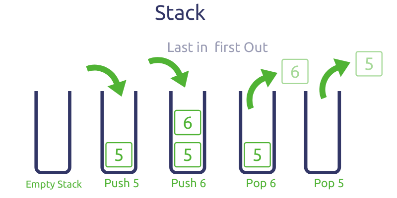
• A stack follows the last in, first out (LIFO) principle. Unlike an array structure, which allows random access at all the positions, a stack limits the insert (push) and remove (pop) operation to only one end of the data structure, i.e., to the top. A stack also allows us to get the top element in \(O(1)\) time.
• Though there isn’t an explicit stack class in Python, we can use a list instead. To follow the LIFO principle, inserting and removing operations both occur at the tail of the list (which emulates the top of the stack).
• We can use append and pop to add and remove elements off the end in amortized \(O(1)\) time (refer Python Time Complexities). Python lists are implemented as dynamic arrays. Once the array is full, Python will allocate more memory for a larger array and copy the old elements to it. Since this reallocation doesn’t happen too often, append will still be \(O(1)\) in most cases. Also, we can index into the list with -1 to get the last element in a list. Basically, the end of the list will be the “top of the stack”.

stack = []       # Empty stack
stack.append(1)  # Push 1 onto stack, current stack: [1]
stack.append(2)  # Push 2 onto stack, current stack: [1,2]
print(stack[-1]) # Print the element at the top, prints "2"
stack.pop()      # Pop 2 off the stack, current stack: [1]

• A wrapper class to emulate a stack using a list is as follows:

class stack:
    # by default pass in [] as the initial value
    def __init__(self, initialVal=[]):
        self.stack = initialVal

    # push is to append to the tail of the list
    def push(self, elem):
        self.stack.append(elem)
        return self.stack

    # pop is to remove from the tail of the list
    def pop(self):
        return self.stack.pop(-1)

    def checkStack(self):
        print(self.stack)

    def checkTop(self):
        print(self.stack[-1])

Queue

• Similar to a stack, a queue also limits the insertion and removal of elements to specific ends of the data structure. However, unlike a stack, a queue follows the first in, first out (FIFO) principle.

• In Python, a queue can also be implemented using a list. In accordance with the FIFO principle, the insertion operation occurs at the tail of the list, while the deletion operation occurs at the head of the list.

• A wrapper class to emulate a queue using a list is as follows:

class queue:
    # by default pass in [] as the initial value
    def __init__(self, initialVal=[]):
        self.queue = initialVal

    # enqueue is to append to the tail of the list
    def enqueue(self, elem):
        self.queue.append(elem)
        return self.queue

    # dequeue is to remove from the head of the list
    def dequeue(self):
        return self.queue.pop(0)

    def checkQueue(self):
        print(self.queue)

    def checkHead(self)
        print(self.queue[0])

    def checkTail(self)
        print(self.queue[-1])

Double-ended Queue (Deque)

• In the collections package, Python provides deque, a double-ended queue class. With deque, we can insert and remove from both ends in \(O(1)\) time. The deque constructor takes in an iterable – we can pass in an empty list to create an empty deque.

from collections import deque
queue = deque([])

• The main methods are append, appendleft, pop and popleft. As the names suggest, append and pop will add and remove elements from the end, whereas appendleft and popleft do the same at the front. In order to emulate a queue, we add from one side and remove from the other.

from collections import deque

queue = deque([])          # Create an empty deque, current deque: []
queue.appendleft(5)        # Add 5 to the front of the queue, current deque: [5]
queue.appendleft(1)        # Add 1 to the front of the queue, current deque: [1, 5]
element = queue.pop()      # Pop 5 from the end of the queue, current deque: [1]
next_element = queue.pop() # Pop 1 from the end of the queue, current deque: []

• If you noticed, we can also use deque to emulate a stack: we add and remove from the same side.

• On a different note, a common mistake is using lists as queues. Let’s consider two ways we can use lists as queues. We can add to the front of the list and remove from the end. This requires using [insert](https://www.tutorialspoint.com/python/list_insert.html) at index 0 and pop.

queue = [2, 3, 4, 5]
queue.insert(0, 1)    # Add 1 at index 0, [1, 2, 3, 4, 5]
element = queue.pop() # Pop 5 from the end, [1, 2, 3, 4]

• The problem is that inserting an element at the front of a list is \(O(N)\), since all the other elements must be shifted to the right (Time Complexity).
• Let’s say instead we decided to add at the end and remove from the front.

queue = [5, 4, 3, 2]
queue.append(1)        # Add 1 to the end, [5, 4, 3, 2, 1]
element = queue.pop(0) # Pop 5 from the front, [4, 3, 2, 1]

• The problem still remains, since popping from the front of the list will be \(O(N)\) as everything to the right must shift to the left.
• Even though using lists as queues is fine if the lists are relatively small, using them over the more efficient deque in an interview setting where time complexity is important is not ideal.

Set

• A set object is an unordered collection of distinct hashable objects. It’s one of Python’s built-in types and allows the dynamic adding and removing of elements, iteration, and operations with another set objects.
• Here’s some operations on a set:

# set initialization by passing in a list
myset = set([1, 2, 3, 3, 3])

# set initialization using {}
myset = {1, 2, 3, 3, 3}

# iteration of set
for ele in myset:
  print(ele)

# check if ele in set:
print(True if ele in myset else False)

# add an element to set:
myset.add(ele)

# remove an element from set
myset.remove(ele)

# get length of the set
print(len(myset))

• Here’s some operations on two sets:

myset1 = {1, 2, 3}
myset2 = {1, 2, 4, 5}

# union
myset = myset1.union(myset2)

# intersection
myset = myset1.intersection(myset2)

# difference
myset = myset1.difference(myset2)

Dictionary

• A dictionary contains mapping information of (key, value) pairs.
• Given a key, the corresponding value can be found in the dictionary. It’s also one of Python’s built-in types. The (key, value) pairs can be dynamically added, removed, and modified. A dictionary also allows iteration through the keys, values, and (key, value) pairs.
• Here’s some operations on a dictionary:

# dictionary initialization using {}
mydict = {'a': 1, 'b': 2}

# add new (key,value) pair
mydict['c'] = 3

# modify existing (key,value) pair
mydict['a'] = 5

# remove (key,value) pair
mydict.pop('a')

# get length of the dictionary
print(len(mydict))

# iteration through keys
for key in mydict.keys():
    print(key)

# iteration through values
for value in mydict.values():
    print(value)

# iteration through (key,value) pairs
for key, value in mydict.items():
    print(key,value)

Linked List

• A linked list is a linear data structure, with the previous node pointing to the next node. It can be implemented by defining a ListNode class.
• Here’s some operations on a linked list:

class ListNode:
    def __init__(self, val):
        self.val = val
        self.next = None

# initiation of linked list
headNode = ListNode(1)
secondNode = ListNode(2)
thirdNode = ListNode(3)

headNode.next = secondNode
secondNode.next = thirdNode

# iterate through the linked list
curNode = headNode
while curNode:
    print(curNode.val)
    curNode = curNode.next

# insert new listnode with value of 5 in between the secondNode and thirdNode
curNode = headNode
while curNode.val != 2:
    curNode = curNode.next
newNode = ListNode(5)
newNode.next = curNode.next
curNode.next = newNode

# remove the listnode with value of 5
curNode = headNode
while curNode.next.val != 5:
    curNode = curNode.next
    curNode.next = curNode.next.next

Binary Tree

• A tree is a nonlinear data structure where each node has at most two children, which are referred to as the left child and the right child.

Concepts

• There are three important properties of trees: height, depth and level, together with edge and path and tree (data structure) on wiki also explains them briefly:

Edge

The connection between one node to another is an edge.

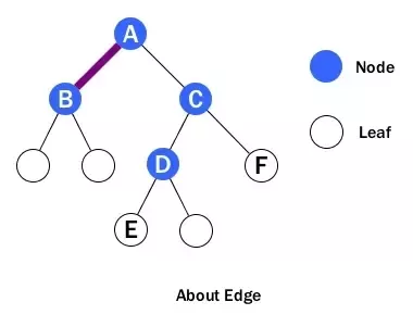
• An example of edge is shown above between A and B. Basically, an edge is a line between two nodes, or a node and a leaf.

Path

A path is a sequence of nodes and edges connecting a node with a descendant.

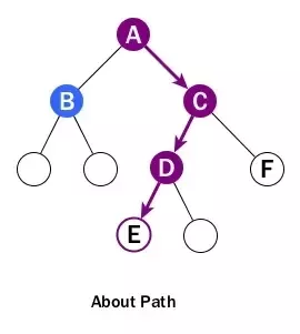
A path starts from a node and ends at another node or a leaf. Please don’t look over the following points:

1. When we talk about a path, it includes all nodes and all edges along the path, not just edges.
2. The direction of a path is strictly from top to bottom and cannot be changed in middle. In the diagram, we can’t really talk about a path from B to F although B is above F. Also there will be no path starting from a leaf or from a child node to a parent node.

Height

The height of a node is the number of edges on the longest downward path between that node and a leaf.

• At first, we can see the above wiki definition has a redundant term - downward - inside. As we already know from previous section, path can only be downward.

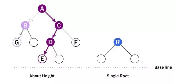
• When looking at height:
  1. Every node has height. So B can have height, so does A, C and D.
  2. Leaf cannot have height as there will be no path starting from a leaf.
  3. It is the longest path from the node to a leaf. So A’s height is the number of edges of the path to E, NOT to G. And its height is 3.
• The height of the root is 1.

The height of a tree is the number of edges on the longest downward path between the root and a leaf. Essentially, the height of a tree is the height of its root. Note that if a tree has only one node, then that node is at the same time the root node and the only leaf node, so the height of the tree is 0. On the other hand, if the tree has no nodes, it’s height is -1.

• Frequently, we may be asked the question: what is the max number of nodes a tree can have if the height of the tree is \(h\)?. Of course the answer is \(2h−1\). When \(h=1\), the number of node inside is 1, which is just the root; also when a tree has just root, the height of the root is 1. Hence, the two inductions match.

• How about giving a height of 0? Then it means we don’t have any node in the tree; but still we may have leaf inside. This is why in most languages, the type of a tree can be a leaf alone.

• Moreover, when we use \(2h−1\) to calculate the max number of nodes, leaves are not taken into account. Leaf is not Node. It carries no key or data, and acts only like a STOP sign. We need to remember this when we deal with properties of trees.

Depth

The depth of a node is the number of edges from the node to the tree’s root node.

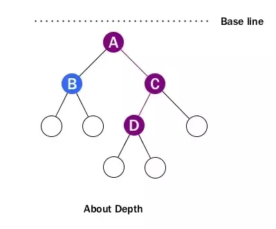
• We don’t care about path any more when depth pops in. We just count how many edges between the targeting node and the root, ignoring directions. For example, D’s depth is 2.

• Recall that when talking about height, we actually imply a baseline located at bottom. For depth, the baseline is at top which is root level. That’s why we call it depth.

• Note that the depth of the root is 0.

The depth of a binary tree is usually used to refer to the height of the tree.

Level

The level of a node is defined by 1 + the number of connections between the node and the root.

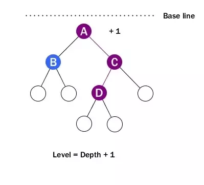
• Simply put, level is depth plus 1.

• The important thing to remember is when talking about level, it starts from 1 and the level of the root is 1. We need to be careful about this when solving problems related to level.

Size

The size of a binary tree is the total number of nodes in that tree.

Example

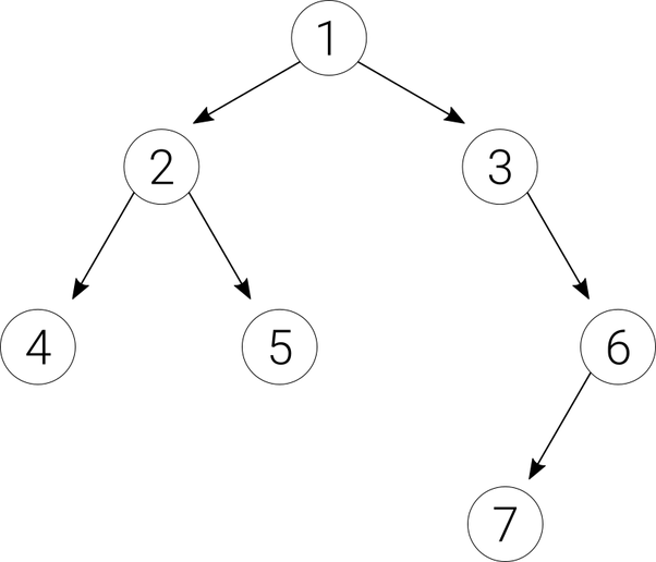
• The height of node 2 is 1 because from 2 there is a path to two leaf nodes (4 and 5), and each of the two paths is only 1 edge long, so the largest is 1.
• The height of node 3 is 2 because from 3 there is a path to only one leaf node (7), and it consists of 2 edges.
• The height of the tree is 3 because from the root node 1 there is a path to three leaf nodes (4, 5, and 7), and the path to the 4 and 5 consists of 2 edges, whereas the path to the 7 consists of 3 edges, so we pick the largest, which is 3.
• The size of the tree is 7.
• The depth of node 2 is 1; The depth of node 3 is 1; the depth node 6 is 2.
• The depth of the binary tree is equal to the height of the tree, so it is 3.

Implementation

• A tree represents the nodes connected by edges. It is a non-linear data structure. It has the following properties −

  • One node is marked as Root node.
  • Every node other than the root is associated with one parent node.
  • Each node can have an arbitrary number of child node.

Create Root

• We just create a Node class and add assign a value to the node. This becomes a tree with only a root node.

class Node:
    def __init__(self, data):
        self.left = None
        self.right = None
        self.data = data
        
    def PrintTree(self):
        print(self.data)

root = Node(10)
root.PrintTree()

• When the above code is executed, it produces the following result −

10

Inserting into a Tree

• To insert into a tree we use the same node class created above and add a insert class to it. The insert class compares the value of the node to the parent node and decides to add it as a left node or a right node. Finally the PrintTree class is used to print the tree.

class Node:
    def __init__(self, data):
        self.left = None
        self.right = None
        self.data = data

    def insert(self, data):
    # Compare the new value with the parent node
        if self.data:
            if data < self.data:
                if self.left is None:
                    self.left = Node(data)
                else:
                    self.left.insert(data)
            elif data > self.data:
                if self.right is None:
                    self.right = Node(data)
               else:
                    self.right.insert(data)
        else:
            self.data = data

    # Print the tree
    def PrintTree(self):
        if self.left:
            self.left.PrintTree()
        print( self.data),
        if self.right:
            self.right.PrintTree()

# Use the insert method to add nodes
root = Node(12)
root.insert(6)
root.insert(14)
root.insert(3)
root.PrintTree()

• When the above code is executed, it produces the following result −

3 6 12 14

Traversing a Tree

• A tree can be traversed by deciding on a sequence to visit each node. We can start at a node then visit the left subtree first and right subtree next, or we can also visit the right subtree first and left subtree next. Accordingly there are different names for these tree traversal methods.

Tree Traversal Algorithms

• Traversal is a process to visit all the nodes of a tree and may print their values too. Because, all nodes are connected via edges (links) we always start from the root (head) node. That is, we cannot randomly access a node in a tree. There are three ways which we use to traverse a tree.
  • In-order Traversal
  • Pre-order Traversal
  • Post-order Traversal

In-order Traversal

• In this traversal method, the left subtree is visited first, then the root and later the right subtree. We should always remember that every node may represent a subtree itself.

• In the below python program, we use the Node class to create place holders for the root node as well as the left and right nodes. Then, we create an insert function to add data to the tree. Finally, the In-order traversal logic is implemented by creating an empty list and adding the left node first followed by the root or parent node.

• At last the left node is added to complete the In-order traversal. Please note that this process is repeated for each subtree until all the nodes are traversed.

class Node:
    def __init__(self, data):
        self.left = None
        self.right = None
        self.data = data
    
    # Insert Node
    def insert(self, data):
        if self.data:
            if data < self.data:
                if self.left is None:
                   self.left = Node(data)
                else:
                   self.left.insert(data)
        else data > self.data:
            if self.right is None:
               self.right = Node(data)
            else:
               self.right.insert(data)
        else:
         self.data = data

    # Print the Tree
    def PrintTree(self):
    if self.left:
        self.left.PrintTree()
    print(self.data),
    if self.right:
        self.right.PrintTree()
     
    # Inorder traversal
    # Left -> Root -> Right
    def inorderTraversal(self, root):
        res = []
        if root:
            res = self.inorderTraversal(root.left)
            res.append(root.data)
            res = res + self.inorderTraversal(root.right)
        return res
        
root = Node(27)
root.insert(14)
root.insert(35)
root.insert(10)
root.insert(19)
root.insert(31)
root.insert(42)
print(root.inorderTraversal(root))      

• When the above code is executed, it produces the following result −

[10, 14, 19, 27, 31, 35, 42]

Pre-order Traversal

• In this traversal method, the root node is visited first, then the left subtree and finally the right subtree.

• In the below python program, we use the Node class to create place holders for the root node as well as the left and right nodes. Then, we create an insert function to add data to the tree. Finally, the Pre-order traversal logic is implemented by creating an empty list and adding the root node first followed by the left node.

• At last, the right node is added to complete the pre-order traversal. Please note that, this process is repeated for each subtree until all the nodes are traversed.

class Node:
   def __init__(self, data):
      self.left = None
      self.right = None
      self.data = data

    # Insert Node
    def insert(self, data):
        if self.data:
            if data < self.data:
                if self.left is None:
                    self.left = Node(data)
                else:
                    self.left.insert(data)
        elif data > self.data:
            if self.right is None:
                self.right = Node(data)
            else:
                self.right.insert(data)
        else:
            self.data = data

    # Print the Tree
    def PrintTree(self):
        if self.left:
            self.left.PrintTree()
      print(self.data),
        if self.right:
            self.right.PrintTree()

    # Preorder traversal
    # Root -> Left ->Right
    def PreorderTraversal(self, root):
        res = []
        if root:
            res.append(root.data)
            res = res + self.PreorderTraversal(root.left)
            res = res + self.PreorderTraversal(root.right)
        return res

root = Node(27)
root.insert(14)
root.insert(35)
root.insert(10)
root.insert(19)
root.insert(31)
root.insert(42)
print(root.PreorderTraversal(root))

• When the above code is executed, it produces the following result −

[27, 14, 10, 19, 35, 31, 42]

Post-order Traversal

• In this traversal method, the root node is visited last, hence the name. First, we traverse the left subtree, then the right subtree and finally the root node.

• In the below python program, we use the Node class to create place holders for the root node as well as the left and right nodes. Then, we create an insert function to add data to the tree. Finally, the Post-order traversal logic is implemented by creating an empty list and adding the left node first followed by the right node.

• At last the root or parent node is added to complete the Post-order traversal. Please note that, this process is repeated for each subtree until all the nodes are traversed.

class Node:
    def __init__(self, data):
        self.left = None
        self.right = None
        self.data = data

    # Insert Node
    def insert(self, data):
        if self.data:
            if data < self.data:
                if self.left is None:
                    self.left = Node(data)
            else:
                self.left.insert(data)
        else if data > self.data:
            if self.right is None:
                self.right = Node(data)
            else:
                self.right.insert(data)
        else:
            self.data = data

    # Print the Tree
    def PrintTree(self):
        if self.left:
            self.left.PrintTree()
        print(self.data),
        if self.right:
            self.right.PrintTree()

# Postorder traversal
# Left ->Right -> Root
def PostorderTraversal(self, root):
    res = []
    if root:
        res = self.PostorderTraversal(root.left)
        res = res + self.PostorderTraversal(root.right)
        res.append(root.data)
    return res

root = Node(27)
root.insert(14)
root.insert(35)
root.insert(10)
root.insert(19)
root.insert(31)
root.insert(42)
print(root.PostorderTraversal(root))

• When the above code is executed, it produces the following result −

[10, 19, 14, 31, 42, 35, 27]

Summary

class TreeNode:
    def __init__(self, val):
        self.val = val
        self.left = None
        self.right = None

# initialization of a tree
rootNode = TreeNode(1)
leftNode = TreeNode(2)
rightNode = TreeNode(3)

rootNode.left = leftNode
rootNode.right = rightNode

# inorderTraversal of the tree (Left, Root, Right)
def inorderTraversal(root):
    result = []

    if not root:
        return self.result

    def df(node: TreeNode):
        if not node:
            return
        df(node.left)
        result.append(node.val)
        df(node.right)

    df(root)
    return result

# preorderTraversal of the tree (Root, Left, Right)
def preorderTraversal(root):
    result = []

    if not root:
        return result

    def df(node: TreeNode):
        if not node:
            return
        result.append(node.val)
        df(node.left)
        df(node.right)

    df(root)
    return result

# postorderTraversal of the tree (Left, Right, Root)
def postorderTraversal(root):
    result = []

    if not root:
        return result

    def df(node: TreeNode):
      if not node:
          return
      df(node.left)
      df(node.right)
      result.append(node.val)

    df(root)
    return result

print('inorder: ', inorderTraversal(rootNode))
print('preorder: ', preorderTraversal(rootNode))
print('postorder: ', postorderTraversal(rootNode))

Heap

heapq for creating min-heaps

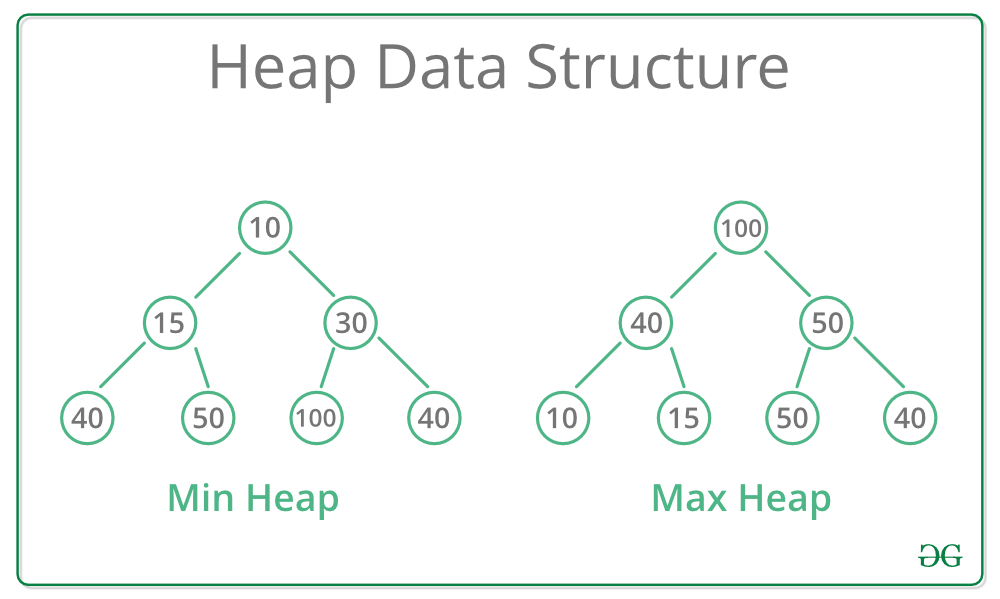
• Similar to stacks, there is no explicit class to create a heap (or a priority queue) in Python. Instead, we have heapq, a collection of methods that allows us to use lists as heaps.

import heapq
heap = [] # Create a new 'heap'. it is really just a list

• We can add elements to our heap with heapq.heappush and pop elements out of our heap with heapq.heappop.

heapq.heappush(heap, 1)       # Push the value 1 into the heap
element = heapq.heappop(heap) # Pop the value on top of the heap: 1. The heap is now empty

• heapq.heappush and heapq.heappop will maintain the min-heap invariant in the list that we use as a heap. As an example:

heap = []
numbers = [9,2,4,1,3,11]
k = 3
ksmallest = []

# Build the heap
for number in numbers:
    heapq.heappush(heap, number)

# Pop k smallest elements
for i in range(k):
    ksmallest.append(heapq.heappop(heap)) # ksmallest is [1,2,3]
    
print(ksmallest) 

• If we were to push all the elements in numbers into heap and pop out 3 times, we would get the 3 smallest elements – in this case [1,2,3]. There is no “setting” that tells the heapq functions to treat our heap as a max-heap: the functions “assume” that the passed in heap is a min-heap and only provide the expected results if it is.

What if you want a max-heap?

• As previously stated, we cannot directly use a max-heap with heapq. Instead, we can try to invert our elements in the min-heap so that the larger elements get popped out first.
• For example, say you have a list of numbers, and want the K largest numbers. To begin, we can invert the numbers by multiplying by -1. The numbers that were the largest are now the smallest. We can now turn this collection of numbers into a min-heap. When we pop our inverted numbers from the heap, we simply multiply by -1 again to get our initial number back.

numbers = [4, 1, 24, 2, 1]

# Invert numbers so that the largest values are now the smallest
numbers = [-1 * n for n in numbers]

# Turn numbers into min heap
heapq.heapify(numbers)

# Pop out 2 times
k = 2
klargest = []
for i in range(k):
    # Multiply by -1 to get our initial number back
    klargest.append(-1 * heapq.heappop(numbers))

# K largest will be [24, 4]

• Thus, in situations where you need a max-heap, consider how you can reverse the order of the elements, turning the largest elements into the smallest.

Building a heap

• As shown above, one approach is to make an additional empty list and push the elements into that list with heapq.heappush. The time complexity of this approach is \(O(N\log{N})\) where \(N\) is the number of elements in the list.
• A more efficient approach is to use heapq.heapify. Given a list, this function will swap its elements in place to make the list a min-heap. Moreover, heapq.heapify only takes \(O(N)\) time.

# Approach 1: push new elements into the heap
numbers = [4, 1, 24, 2, 1]
heap = [] # our "heap"
for num in numbers:
    heapq.heappush(heap, num)
smallest_num = heapq.heappop(heap)
# Time complexity: O(nlogn)

# Approach 2: use heapify()
numbers = [4, 1, 24, 2, 1]
heapq.heapify(numbers) # numbers can act as our heap now'. 
smallest_num = heapq.heappop(numbers)
# Time complexity: O(n)

Comparing across multiple fields

• Suppose we had the age and height (in inches) of students stored in a list.

# each entry is a tuple (age, height)
students = [(12, 54), (18, 78), (18, 62), (17, 67), (16, 67), (21, 76)]

• Let’s say we wanted to get the K youngest students, and if two students had the same age, let’s consider the one who is shorter to be younger. Unfortunately, there is no way for us to use a custom comparator function to handle cases where two students have the same age. Instead, we can use tuples to allow the heapq functions to compare multiple fields. To provide an example, consider the students at indices 0 and 1. Since, student 0’s age, 12, is less than student 1’s, 18, student 0 will be considered smaller and will be closer to the top of the heap than student 1. Let’s now consider student 1 and student 2. Since both of their ages are the same, the heapq functions will compare the next field in the tuple, which is height. Student 2 has a smaller height, so student 2 will be considered smaller and will be closer to the top.

# Each entry is a tuple (age, height)
students = [(12, 54), (18, 78), (18, 62), (17, 67), (16, 67), (21, 76)]

# Since our student ages and heights are already tuples, no need to pre-process
heapq.heapify(students)

k = 4
kyoungest = []
for i in range(k):
    kyoungest.append(heapq.heappop(students))

# K youngest will be [(12, 54), (16, 67), (17, 67), (18, 62)]

• If you need to compare against multiple fields to find out which element is smaller or bigger, consider having the heap’s elements be tuples.

Trie

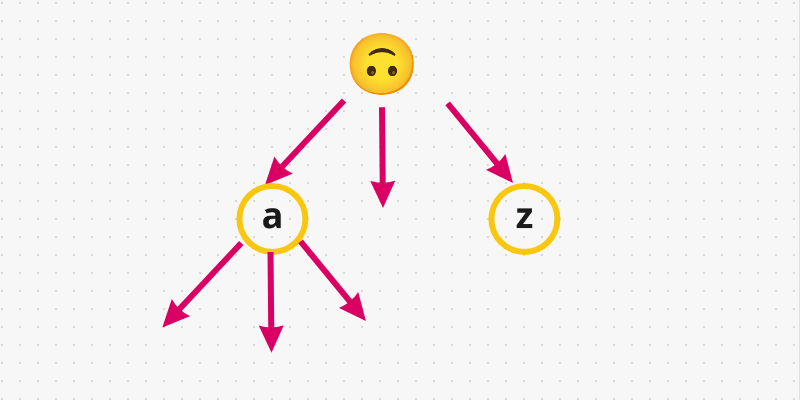
• Let’s understand Trie first. Trie is basically a tree where each node holds a character and can have up to 26 children in the word add-search context, because we have 26 lower case characters in the alphabet (from a to z). So, basically each node represents a single character. Graphically speaking:

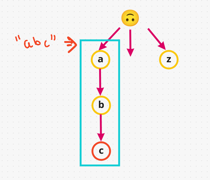
• If we insert the word abc in our trie, a will have b as a child, which in turn will have c as a child. Graphically, this is how it looks like:

• Note that in the above example, c denotes the end of the word for the word abc. Now, if we added another word example, say ab, we don’t add a and b back again since they are already available to us. We can simply re-use these characters. So, we have two words along this path abc and ab. Basically, all words that start with a and b would live in this space, that’s what makes it efficient. Hence, a trie is also called a prefix tree.

• Now let’s take an example and build our tree.

Input
["WordDictionary","addWord","addWord","addWord","search","search","search","search"]
[[],["bad"],["dad"],["mad"],["pad"],["bad"],[".ad"],["b.."]]

Output
[null,null,null,null,false,true,true,true]

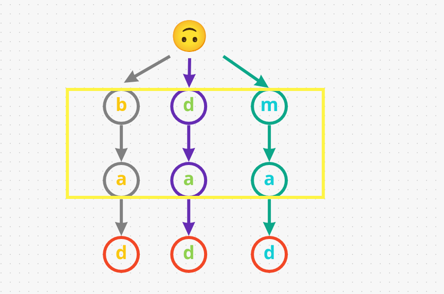
• The first word we add is bad, i.e., b -> a -> d.

• Next, let’s add another word dad. Given that we don’t share the same prefix as the earlier word bad (bad starts with b, while dad starts with d), we have to start with a different path. So, let’s add dad as d -> a -> d.

• We have one last word before we start searching, say mad. So, we don’t have m, then let’s add it: m -> a -> d

• So far we have three word’s and all of them end with a different d. But all three of them have different prefixes that’s why they are along different path’s:

• Now let’s look at the searching path:

  • The first word we gonna search for is pad. We start at the root and and begin looking for the first character in the word, i.e., p. We immediately return False as p doesn’t even exist in our input.
  • Now, let’s search for another word bad. We start at the root and see there are any nodes with b. Yes, we have b. Now let’s check does b have a child a, which it does. For the last character d, let’s check if a has a child d, and surely it does! Lastly we have to say the last character d is in our Trie, which designated as the end of the word (marked red in the diagram below). Therefore, we return True for the input bad.
  • Let’s search for .ad next. The dot . character matches any character. We start at the root and go through all possible paths using a DFS or backtracking approach. So, let’s say we start with going down b as the first node. Check if b has a child a, which it does. Now, check if a has a child d, which it also does. Lastly, note that the last character d in our Trie is designated as the end of the word. Therefore, we return True for this input .ad.
  • Let’s try one last search, looking for b... So, we start at the root and see there are any nodes with b. Yes, we have b. Now, check if we have a character under b to match ., which we have as a. Now, we’re looking for a character for our last dot .. Yes we have d and it is the end of the word. Therefore, we return True for this input b...

• Here’s a visual demonstration for the overall process:

Dictionary

• Dictionaries are the Python equivalent to Hash Maps and are an overpowered data structure. In most cases, we can look up, add, delete and update keys in \(O(1)\) time. Let’s go over the basics of dictionaries.

# empty dict
d = {}
# dict with some keys and values
d = {
    "name": "James",
    "age": 29
    5: 29.3
}

• When declaring a dictionary, we put the keys on the left and values on the right, separated by a colon. In Python, the keys of a dictionary can only be hashable values, like int, str, tuple, and more (Hashable Objects). In addition, a dictionary can have keys and values of multiple types as shown above.

• We can also add, update and delete keys with [].

d["numbers"] = [1, 2, 4, 12] # add key "numbers" to d
d["numbers"] = [1, 3, 6, 18] # update key "numbers" of d
del d["numbers"] # delete key "numbers" of d

• We can also easily check if a key is in a dictionary with in.

doesNumbersExist = "numbers" in d

• Python also provides a nice way of iterating over the keys inside a dictionary.

d = {"a": 0, "b": 5, "c": 6, "d": 7, "e": 11, "f": 19}

# iterate over each key in d
for key in d:
    print(d[key])

• When you are iterating over keys in this manner, remember that you cannot add new keys or delete any existing keys, as this will result in an error.

Accessing a non-existent key

d = {"a": 0, "b": 7}
c_count = d["c"] # KeyError: 'c'

• In the above snippet, c does not exist. We will get a KeyError when we run the code. As a result, in many situations, we need to check if the key exists in a dictionary before we try to access it.
• Although this check is simple, it can be a hassle in an interview if we need to do it many times. Alternatively, if we use collections.defaultdict, there is no need for this check. defaultdict operates in the same way as a dictionary in nearly all aspects except for handling missing keys. When accessing keys that don’t exist, defaultdict automatically sets a default value for them. The factory function to create the default value can be passed in the constructor of defaultdict.

from collections import defaultdict

# create an empty defaultdict with default value equal to []
default_list_d = defaultdict(list)
default_list_d['a'].append(1) # default_list_d is now {"a": [1]}

# create a defaultdict with default value equal to 0
default_int_d = defaultdict(int)
default_int_d['c'] += 1       # default_int_d is now {"c": 1}

• We can also pass in a lambda as the factory function to return custom default values. Let’s say for our default value we return the tuple (0, 0).

pair_dict = defaultdict(lambda: (0,0)) 
print(pair_dict['point'] == (0,0)) # prints True

• Using a defaultdict can help reduce the clutter in your code, speeding up your implementation.

Graph

• A graph is a data structure that consists of the following two components:
  1. A finite set of vertices/nodes.
  2. A finite set of an ordered pair of the form (u, v) called as edges/arcs. The pair is ordered because (u, v) is not the same as (v, u) in case of a directed graph (di-graph). The pair of the form (u, v) indicates that there is an edge from vertex u to vertex v. The edges may contain weight/value/cost.
• Graphs are used to represent many real-life applications. Graphs are used to represent networks. The networks may include paths in a city, a telephone network, a circuit network etc. Graphs are also used in social networks such as LinkedIn, Facebook. For example, in Facebook, each person is represented with a vertex (or node). Each node is a structure and contains information such as the person’s ID, name, gender, and locale. See this for more applications of graph.
• The following is an example of an undirected graph with five vertices:

• The following two are the most commonly used representations of a graph:
  1. Adjacency Matrix
  2. Adjacency List
• There are other representations also such as the Incidence Matrix and Incidence List. The choice of graph representation is situation-specific and depends on the type of operations to be performed and ease of use of each graph representation type.

Adjacency Matrix

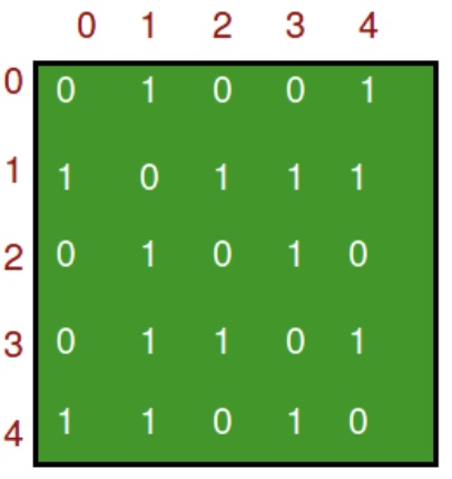
• An adjacency matrix is a 2D array of size \(V \times V\) where \(V\) is the number of vertices in a graph. Let the 2D array be adj[][], a slot adj[i][j] = 1 indicates that there is an edge from vertex i to vertex j. Adjacency matrix for an undirected graph is always symmetric. Adjacency matrix is also used to represent weighted graphs. If adj[i][j] = w, then there is an edge from vertex i to vertex j with weight w.

• The adjacency matrix for the above example graph is:

• Pros:
  • Representation is easier to implement and follow.
  • Removing an edge takes \(O(1)\) time. Queries such as checking whether there is an edge from vertex \(u\) to vertex v are efficient and can be done \(O(1)\).
• Cons:
  • Inefficient in terms of the space requirements, since it consumes \(O(V^2)\) space. Even if the graph is sparse (i.e., it contains less number of edges), it still consumes the same space. Adding a vertex takes \(O(V^2)\) time. Computing all neighbors of a vertex takes \(O(V)\) time (thus, inefficient).
• Please see this for a sample Python implementation of adjacency matrix.

Adjacency List

• An array of lists is used. The size of the array is equal to the number of vertices. Let the array be an array[]. An entry array[i] represents the list of vertices adjacent to the \(i^{th}\) vertex. This representation can also be used to represent a weighted graph. The weights of edges can be represented as lists of pairs. Following is the adjacency list representation of the above graph:

• Here’s a Python implementation using a list (which is internally implemented using a dynamic array) to represent adjacency lists instead of the linked list. The dynamic array implementation of lists offers the distinct advantage of cache friendliness (for sequential accesses) compared to linked lists.

"""
A Python program to demonstrate the adjacency
list representation of the graph
"""
 
# A class to represent the adjacency list of the node
 
 
class AdjNode:
    def __init__(self, data):
        self.vertex = data
        self.next = None
 
 
# A class to represent a graph. A graph
# is the list of the adjacency lists.
# Size of the array will be the no. of the
# vertices "V"
class Graph:
    def __init__(self, vertices):
        self.V = vertices
        self.graph = [None] * self.V
 
    # Function to add an edge in an undirected graph
    def add_edge(self, src, dest):
        # Adding the node to the source node
        node = AdjNode(dest)
        node.next = self.graph[src]
        self.graph[src] = node
 
        # Adding the source node to the destination as
        # it is the undirected graph
        node = AdjNode(src)
        node.next = self.graph[dest]
        self.graph[dest] = node
 
    # Function to print the graph
    def print_graph(self):
        for i in range(self.V):
            print("Adjacency list of vertex {}\n head".format(i), end="")
            temp = self.graph[i]
            while temp:
                print(" -> {}".format(temp.vertex), end="")
                temp = temp.next
            print(" \n")
 
 
# Driver program to the above graph class
if __name__ == "__main__":
    V = 5
    graph = Graph(V)
    graph.add_edge(0, 1)
    graph.add_edge(0, 4)
    graph.add_edge(1, 2)
    graph.add_edge(1, 3)
    graph.add_edge(1, 4)
    graph.add_edge(2, 3)
    graph.add_edge(3, 4)
 
    graph.print_graph()

• which outputs:

Adjacency list of vertex 0
head -> 1-> 4

Adjacency list of vertex 1
head -> 0-> 2-> 3-> 4

Adjacency list of vertex 2
head -> 1-> 3

Adjacency list of vertex 3
head -> 1-> 2-> 4

Adjacency list of vertex 4
head -> 0-> 1-> 3

• Pros:
  • Saves space since it needs \(O(\|V\|+\|E\|)\) space. In the worst case, there can be \(C(V, 2)\) number of edges in a graph thus consuming \(O(V^2)\) space. Adding a vertex is easier than an adjacency matrix. Computing all neighbors of a vertex takes optimal time.
• Cons:
  • Queries like whether there is an edge from vertex \(u\) to vertex \(v\) are inefficient and need \(O(V)\) time.

In real-life problems, graphs are sparse (i.e., \(|E| << |V|^2\)). That’s why adjacency lists are commonly used for storing graphs since an adjacency matrix enforces a $$

V

^2$$ bound on time complexity.

• For more, refer Wikipedia: Graph (abstract data type).

Generate a graph using Dictionary in Python

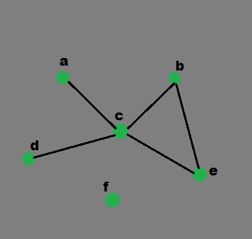
• Let’s see how to implement a graph in python using the dictionary data structure in python. The keys of the dictionary are the nodes/vertices of our graph and the corresponding values are lists that contain nodes, each of which are connected to the original node by an edge/arc.
• The keys of the dictionary used are the nodes of our graph and the corresponding values are lists with each nodes, which are connecting by an edge. This simple graph has six nodes (a-f) and five arcs:

a -> c
b -> c
b -> e
c -> a
c -> b
c -> d
c -> e
d -> c
e -> c
e -> b

• It can be represented by the following Python data structure. This is a dictionary whose keys are the nodes of the graph. For each key, the corresponding value is a list containing the nodes that are connected by a direct arc from this node.

graph = { "a" : ["c"],
          "b" : ["c", "e"],
          "c" : ["a", "b", "d", "e"],
          "d" : ["c"],
          "e" : ["c", "b"],
          "f" : []
        } 

• Graphical representation of above example:

• defaultdict: Usually, a Python dictionary throws a KeyError if you try to get an item with a key that is not currently in the dictionary. defaultdict allows that if a key is not found in the dictionary, then instead of a KeyError being thrown, a new entry is created. The type of this new entry is given by the argument of defaultdict.

Generate graph

# Python program for
# validation of a graph
 
# import dictionary for graph
from collections import defaultdict
 
# function for adding edge to graph
graph = defaultdict(list)
def addEdge(graph,u,v):
    graph[u].append(v)
 
# definition of function
def generate_edges(graph):
    edges = []
 
    # for each node in graph
    for node in graph:
         
        # for each neighbour node of a single node
        for neighbour in graph[node]:
             
            # if edge exists then append
            edges.append((node, neighbour))
    return edges
 
# declaration of graph as dictionary
addEdge(graph,'a','c')
addEdge(graph,'b','c')
addEdge(graph,'b','e')
addEdge(graph,'c','d')
addEdge(graph,'c','e')
addEdge(graph,'c','a')
addEdge(graph,'c','b')
addEdge(graph,'e','b')
addEdge(graph,'d','c')
addEdge(graph,'e','c')
 
# Driver Function call
# to print generated graph
print(generate_edges(graph))

• which outputs:

[('a', 'c'), ('c', 'd'), ('c', 'e'), ('c', 'a'), ('c', 'b'), 
('b', 'c'), ('b', 'e'), ('e', 'b'), ('e', 'c'), ('d', 'c')]

• Note that since we have taken example of an undirected graph, we print the same edge twice say as (‘a’,’c’) and (‘c’,’a’). This issue can be fixed using a directed graph.

Generate the path from one node to the other node

• Using Python dictionary, we can find the path from one node to the other in a Graph. The idea is similar to DFS in graphs.
• In the function, initially, the path is an empty list. In the starting, if the start node matches with the end node, the function will return the path. Otherwise the code goes forward and hits all the values of the starting node and searches for the path using recursion.

# Python program to generate the first
# path of the graph from the nodes provided
 
graph = {
    'a': ['c'],
    'b': ['d'],
    'c': ['e'],
    'd': ['a', 'd'],
    'e': ['b', 'c']
}
 
# function to find path
def find_path(graph, start, end, path=[]):
    path = path + [start]
    if start == end:
        return path
    for node in graph[start]:
        if node not in path:
            newpath = find_path(graph, node, end, path)
            if newpath:
                return newpath
 
# Driver function call to print the path
print(find_path(graph, 'd', 'c'))

• which outputs:

['d', 'a', 'c']

Generate all the possible paths from one node to the other

• Let’s generate all the possible paths from the start node to the end node. The basic functioning works same as the functioning of the above code. The place where the difference comes is instead of instantly returning the first path, it saves that path in a list named as paths in the example below.
• Finally, after iterating over all the possible ways, it returns the list of paths. If there is no path from the starting node to the ending node, it returns None.

# Python program to generate the all possible
# path of the graph from the nodes provided
graph ={
'a':['c'],
'b':['d'],
'c':['e'],
'd':['a', 'd'],
'e':['b', 'c']
}
 
# function to generate all possible paths
def find_all_paths(graph, start, end, path =[]):
  path = path + [start]
  if start == end:
    return [path]
  paths = []
  for node in graph[start]:
    if node not in path:
      newpaths = find_all_paths(graph, node, end, path)
    for newpath in newpaths:
      paths.append(newpath)
  return paths
   
# Driver function call to print all
# generated paths
print(find_all_paths(graph, 'd', 'c'))

• which outputs:

[['d', 'a', 'c'], ['d', 'a', 'c']]

Generate the shortest path

• To get to the shortest from all the paths, we use a little different approach as shown below. In this, as we get the path from the start node to the end node, we compare the length of the path with a variable named as shortest which is initialized with the None value.
• If the length of generated path is less than the length of shortest, if shortest is not None, the newly generated path is set as the value of shortest. Again, if there is no path, it returns None.

# Python program to generate shortest path
 
graph ={
'a':['c'],
'b':['d'],
'c':['e'],
'd':['a', 'd'],
'e':['b', 'c']
}
 
# function to find the shortest path
def find_shortest_path(graph, start, end, path =[]):
        path = path + [start]
        if start == end:
            return path
        shortest = None
        for node in graph[start]:
            if node not in path:
                newpath = find_shortest_path(graph, node, end, path)
                if newpath:
                    if not shortest or len(newpath) < len(shortest):
                        shortest = newpath
        return shortest
         
# Driver function call to print
# the shortest path
print(find_shortest_path(graph, 'd', 'c'))

• which outputs:

['d', 'a', 'c']

Python Time Complexities

• This page documents the time-complexity (aka “Big O” or “Big Oh”) of various operations in current CPython. Other Python implementations (or older or still-under development versions of CPython) may have slightly different performance characteristics. However, it is generally safe to assume that they are not slower by more than a factor of \(O(log n)\).

• Generally, \(n\) is the number of elements currently in the container. \(k\) is either the value of a parameter or the number of elements in the parameter.

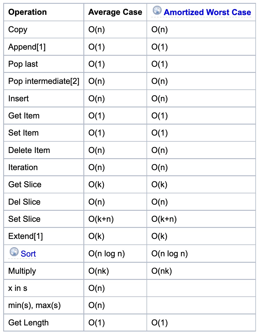
list

• The average case assumes parameters generated uniformly at random.

• Internally, a list is represented as an array; the largest costs come from growing beyond the current allocation size (because everything must move), or from inserting or deleting somewhere near the beginning (because everything after that must move). Note that slicing a list is \(O(k)\) where \(k\) is the length of the slice (since slicing is just “copying part of the list” so the time complexity is the same as a copy). If you need to add/remove at both ends, consider using a collections.deque instead.

string

• Note that since strings are immutable, a new string is created whenever an operation on the input string (say, str.replace()) is performed. Further, similar to lists, slicing a string is \(O(k)\) where \(k\) is the length of the slice (since slicing is just “copying part of the string” so the time complexity is the same as a copy). A string is also an iterable, so the time complexities are for other usual operations are similar to that of a list.

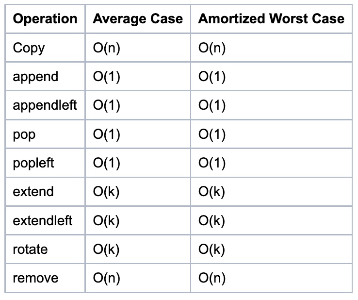
collections.deque

• A deque (double-ended queue) is represented internally as a doubly linked list. (Well, a list of arrays rather than objects, for greater efficiency.) Both ends are accessible, but even looking at the middle is slow, and adding to or removing from the middle is slower still.

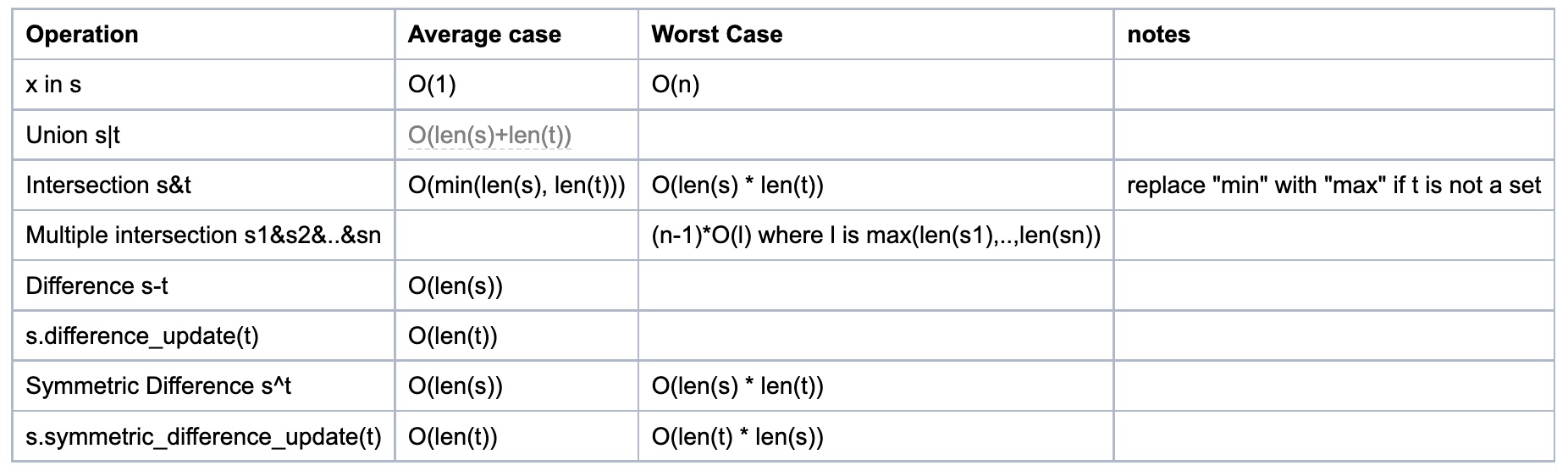
set

• See dict – the implementation is intentionally very similar.

• As seen in the source code the complexities for set difference s-t or s.difference(t) (set_difference()) and in-place set difference s.difference_update(t) (set_difference_update_internal()) are different! The first one is \(O(len(s))\) (for every element in s add it to the new set, if not in t). The second one is \(O(len(t))\) (for every element in t remove it from s). So care must be taken as to which is preferred, depending on which one is the longest set and whether a new set is needed.

• To perform set operations like s-t, both s and t need to be sets. However you can do the method equivalents even if t is any iterable, for example s.difference(l), where l is a list.

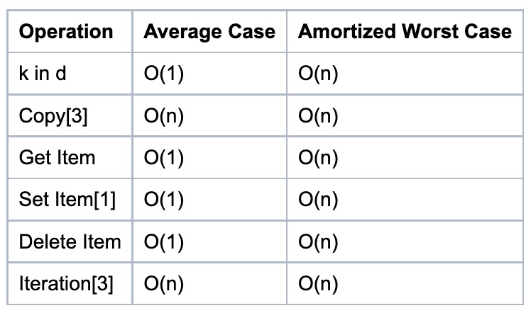
dict

• The average case times listed for dict objects assume that the hash function for the objects is sufficiently robust to make collisions uncommon. The average case assumes the keys used in parameters are selected uniformly at random from the set of all keys.

• Note that there is a fast-path for dicts that (in practice) only deal with str keys; this doesn’t affect the algorithmic complexity, but it can significantly affect the constant factors: how quickly a typical program finishes.

Counter

• collections.Counter is just a subclass of dict. Constructing it is O(n), because it has to iterate over the input, but operations on individual elements remain O(1).

Notes

• [1] = These operations rely on the “Amortized” part of “Amortized Worst Case”. Individual actions may take surprisingly long, depending on the history of the container.
• [2] = Popping the intermediate element at index k from a list of size n shifts all elements after \(k\) by one slot to the left using memmove. \(n - k\) elements have to be moved, so the operation is \(O(n - k)\). The best case is popping the second to last element, which necessitates one move, the worst case is popping the first element, which involves \(n - 1\) moves. The average case for an average value of \(k\) is popping the element the middle of the list, which takes \(O(n/2) = O(n)\) operations.
• [3] = For these operations, the worst case \(n\) is the maximum size the container ever achieved, rather than just the current size. For example, if N objects are added to a dictionary, then \(N-1\) are deleted, the dictionary will still be sized for \(N\) objects (at least) until another insertion is made.

References

• Python Implementations of Data Structures
• Python Dictionary Tips
• What are the differences between type() and isinstance()?
• Quora: What is the height, size, and depth of a binary tree?
• What is the time complexity of collections.Counter() in Python?
• Python Time Complexity
• Big-O of list slicing
• What is the time complexity of slicing a list?
• Graph and its representations
• Generate a graph using Dictionary in Python

Citation

If you found our work useful, please cite it as:

@article{Chadha2020DistilledPythonDS,
  title   = {Python Data Structures and Time Complexities},
  author  = {Chadha, Aman},
  journal = {Distilled AI},
  year    = {2020},
  note    = {\url{https://aman.ai}}
}