Distilled • LeetCode • Asymptotic Notations
- What are Asymptotic Notations?
- (Inefficient) Alternatives
- Types of Asymptotic Notations
- Books
- Online Resources
What are Asymptotic Notations?
- Asymptotic notations allow us to analyze an algorithm’s running time as the input size for the algorithm increases. This is also known as an algorithm’s growth rate.
- Asymptotic notations helps us answer the following questions:
- Does the algorithm suddenly become incredibly slow when the input size grows?
- Does it mostly maintain its quick runtime as the input size increases?
(Inefficient) Alternatives
- One way would be to count the number of primitive operations at different input sizes.
- (-) Though this is a valid solution, the amount of work this takes for even simple algorithms is unjustifiable.
- Another way is to physically measure the amount of time an algorithm takes to complete given different input sizes.
- (-) However, the accuracy of this method is bound to environmental variables such as the underlying hardware infrastructure’s processing power, etc. In other words, the measured times would only be relative to the machine they were computed on.
Types of Asymptotic Notations
- In the initial section on What are Asymptotic Notations?”, we described how an asymptotic notation identifies the behavior of an algorithm as the input size changes. Let us imagine an algorithm as a function \(f\), \(n\) as the input size, and \(f(n)\) being the runtime of the algorithm. So for a given algorithm \(f\) with input size \(n\), you get some resultant runtime \(f(n)\).
- This results in a graph where the Y-axis is the runtime, the X-axis is the input size, and the plot points are the runtime for a given input size.
- You can label a function, or algorithm, with an asymptotic notation in many different ways – you can describe an algorithm by its best case, worst case, or average case. However, the most common is to analyze an algorithm by its worst case.
They say, “plan for the worst and hope for the best”.
- You typically don’t evaluate using the best case because those conditions should not be what you’re planning for. An excellent example of this is sorting algorithms; particularly, adding elements to a tree structure. The best case for most algorithms could be as low as a single operation. However, in some cases, the element you’re adding needs to be sorted appropriately through the tree, which could mean examining an entire branch. This is the worst case, and this is what we plan for.
Types of Functions, Limits and Simplification
| Function | Form |
|---|---|
| Logarithmic | \(\log{n}\) |
| Linear | \(a{\cdot}n + b\) |
| Quadratic | \(a{\cdot}n^2 + b{\cdot}n + c\) |
| Polynomial | \(a{\cdot}n^z + \ldots + a{\cdot}n^2 + a{\cdot}n^1 + a{\cdot}n^0, \text{where z is some constant}\) |
| Exponential | \(a^n, \text{where a is some constant}\) |
- These are some fundamental function growth classifications used in various notations. The list starts at the slowest growing function (logarithmic, fastest execution time) and goes on to the fastest growing (exponential, slowest execution time). Note that as \(n\) increases for each of those functions, the result increases much quicker in quadratic, polynomial, and exponential, compared to logarithmic and linear.
- It is worth noting that for the notations about to be discussed, you should do your best to use the simplest terms. This means to disregard:
- Constants
- Lower order terms
- This is because as the input size (or \(n\) in our \(f(n)\) example) grows, and tends to \(\infty\), the lower order terms and constants are of little to no importance. That being said, if you have constants that are huge (read: a ridiculous, unimaginable amount), realize that simplifying skews your notation accuracy.
- Since we want the simplest “base” form, let’s update our table a bit:
| Function | Form |
|---|---|
| Logarithmic | \(\log{n}\) |
| Linear | \(n\) |
| Quadratic | \(n^2\) |
| Polynomial | \(n^z, \text{where z is some constant}\) |
| Exponential | \(a^n, \text{where a is some constant}\) |
Big-O
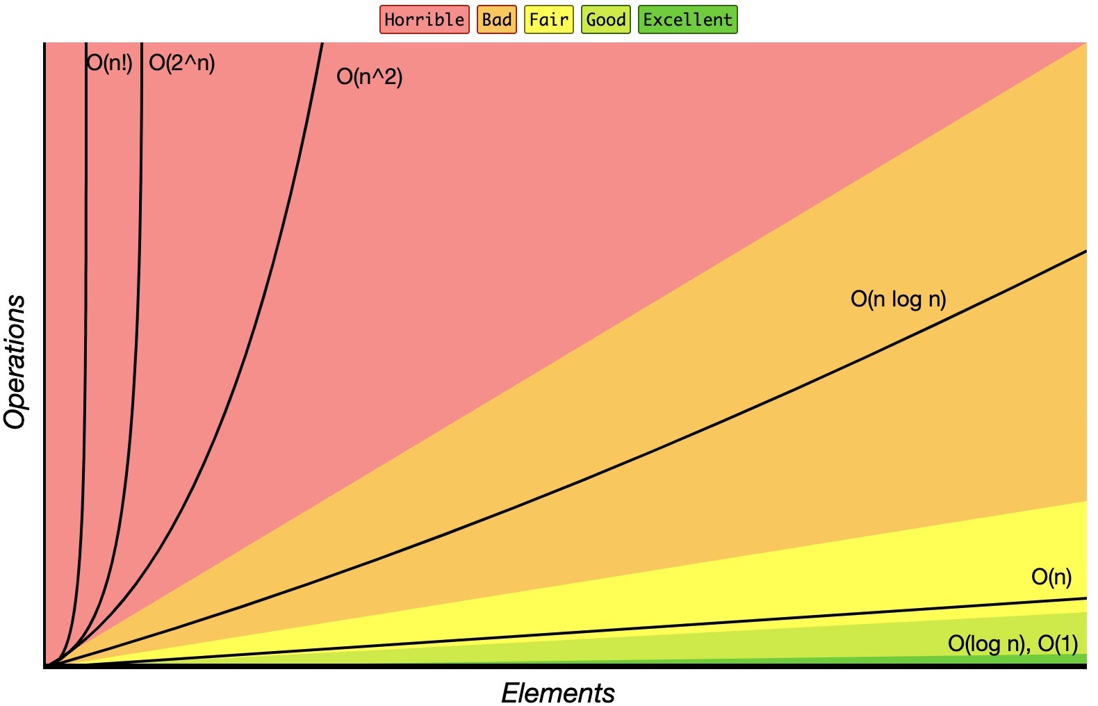
- Big-O, commonly written as O, is an asymptotic notation for the worst case, or ceiling of growth for a given function. It provides us with an asymptotic upper bound for the growth rate of the runtime of an algorithm.
- Say \(f(n)\) is your algorithm runtime, and \(g(n)\) is an arbitrary time complexity you are trying to relate to your algorithm. \(f(n)\) is \(O(g(n)\), if for some real constants \(c (c > 0)\) and \(n_0\), \(f(n) <= c \cdot g(n)\) for every input size \(n\) \((n > n_0)\).
- Big-O is the primary notation used for general algorithm time complexity.
- The diagram below from Big-O Cheat Sheet illustrates what a Bio-O time complexity chart looks like with a range of standard complexities.
Example 1
\[f(n) = 3 \cdot \log{n} + 100 \\ g(n) = \log{n}\]Is \(f(n)\) \(O(g(n))?\)
- Using the definition of Big-O,
- Is there some pair of constants \(c\), \(n_0\) that satisfies this for all \(n > n_0?\)
- Yes! The definition of Big-O has been met therefore \(f(n)\) is \(O(g(n))\).
Example 2
\[f(n) = 3 \cdot n^2\\ g(n) = n\]Is \(f(n)\) \(O(g(n))?\)
- Using the definition of Big-O,
- Is there some pair of constants \(c\), \(n_0\) that satisfies this for all \(n > 0?\)
- No, there isn’t. Thus, \(f(n)\) is NOT \(O(g(n))\).
Big-Omega
- Big-Omega, commonly written as \(\Omega\), is an asymptotic notation for the best case, or a floor growth rate for a given function. It provides us with an asymptotic lower bound for the growth rate of the runtime of an algorithm.
- \(f(n)\) is \(Ω(g(n))\), if for some real constants \(c (c > 0)\) and \(n_0\) \((n_0 > 0)\), \(f(n)\) is \(\geq c {\cdot} g(n)\) for every input size \(n\) \((n > n_0)\).
- Note:
- The asymptotic growth rates provided by big-O and big-omega notation may or may not be asymptotically tight.
- Thus we use small-o and small-omega notation to denote bounds that are not asymptotically tight, which we delve into in the below sections.
Small-o
- Small-o, commonly written as \(o\), is an asymptotic notation to denote the upper bound (that is not asymptotically tight) on the growth rate of the runtime of an algorithm.
- \(f(n)\) is \(o(g(n))\), if for all real constants \(c (c > 0)\) and \(n_0\) \((n_0 > 0)\), \(f(n)\) is < \(c \cdot g(n)\) for every input size \(n\) \((n > n_0)\).
- The definitions of O-notation and o-notation are similar. The main difference is that in \(f(n) = O(g(n))\), the bound \(f(n) \leq g(n)\) holds for some constant \(c > 0\), but in \(f(n) = o(g(n))\), the bound \(f(n) < c \cdot g(n)\) holds for all constants \(c > 0\).
Small-omega
- Small-omega, commonly written as \(\omega\), is an asymptotic notation to denote the lower bound (that is not asymptotically tight) on the growth rate of the runtime of an algorithm.
- \(f(n)\) is \(\omega(g(n))\), if for all real constants \(c (c > 0)\) and \(n_0 (n_0 > 0)\), \(f(n)\) is \(> c \cdot g(n)\) for every input size \(n (n > n_0)\).
- The definitions of \(\Omega\)-notation and \(\omega\)-notation are similar. The main difference is that in \(f(n) = Ω(g(n))\), the bound \(f(n) >= g(n)\) holds for some constant \(c > 0\), but in \(f(n) = \omega(g(n))\), the bound \(f(n) > c \cdot g(n)\) holds for all constants \(c > 0\).
Theta
- Theta, commonly written as \(\theta\), is an asymptotic notation to denote the asymptotically tight bound on the growth rate of the runtime of an algorithm.
- \(f(n)\) is \(\theta(g(n))\), if for some real constants \(c_1, c_2\) and \(n_0\) \((c_1 > 0, c_2 > 0, n_0 > 0)\), \(c_1 \cdot g(n)\) is < \(f(n)\) is < \(c_2 \cdot g(n)\) for every input size \(n (n > n_0)\).
- Therefore, \(f(n)\) is \(\theta(g(n))\) implies \(f(n)\) is \(O(g(n))\) as well as \(f(n)\) is \(\Omega(g(n))\).
Endnotes
It’s hard to keep this kind of topic short, and you should go through the books and online resources listed. They go into much greater depth with definitions and examples.
Books
- Introduction to Algorithms by CLRS
- Algorithms by Robert Sedgewick
- Algorithm Design by Michael Goodrich and Roberto Tamassia
Online Resources
- MIT: Big-O Lecture
- KhanAcademy
- Big-O Cheatsheet - common structures, operations and algorithms, ranked by complexity.